

A couple of days ago news about DALL-E 2 and its ability to create realistic images from text descriptions took the world by storm. Even though, this news left me amazed I was hardly surprised. For a while now, machine learning and deep learning are dominating the computer vision field, and engineers are coming up with more and more interesting solutions.
From Facebook tag suggestions to self-driving cars neural networks really took over this world. In fact, the revival of AI 10 years ago started with its application in computer vision. Namely, in a computer vision problem called image classification. Today, we can solve that problem using JavaScript in the browser. Let’s see how we can do that.

This bundle of e-books is specially crafted for beginners.
Everything from Python basics to the deployment of Machine Learning algorithms to production in one place.
Become a Machine Learning Superhero TODAY!
In this article we cover:
- What is Image Classification?
- Convolutional Neural Networks – Neural Networks for Image Classification (and more)
- Dataset and Installation of TensorFlow.js
- Loading and preparing data
- Implementation of Image Classification with Tensorflow.js
1. What is Image Classification?
Image Classification, or sometimes called Image Recognition, is the task of associating one or more labels to a given image, based on the objects that appear in the image. If we are assigning just one label we are talking about single-label classification, and if we are assigning multiple labels to an image we are talking about multiple-label classification.
Historically, image classification is a problem that popularized deep neural networks especially visual types of neural networks – Convolutional neural networks (CNN). We will go into details about what are CNNs and how they work in next section. However, we can say that CNNs were popularized after they broke a record in The ImageNet Large Scale Visual Recognition Challenge (ILSVRC) back in 2012.

This competition evaluates algorithms for object detection and image classification at a large scale. The dataset that they provide contains 1000 image categories and over 1.2 million images. The goal of the image classification algorithm is to correctly predict to which class the object belongs to. Since 2012. every winner of this competition used CNNs.
2. Convolitional Neural Networks – Neural Networks for Image Classification (and more)
This type of neural networks was created back in the 1990s by Yann LeCun, today’s director of AI research at Facebook. Similar to other ideas in the field, this one also has roots in biology. Researchers detected that individual neurons from visual cortex respond to stimuli only in a restricted region of the visual field known as the receptive field.
Because these fields of different neurons overlap, together they make the entire visual field. This effectively means that certain neurons are activated only if there is a certain attribute in the visual field, for example, horizontal edge. So, different neurons will be “fired up” if there is a horizontal edge in your visual field, and different neurons will be activated if there is, let’s say a vertical edge in our visual field.
For example, take a look at this image, and tell us what do you see:
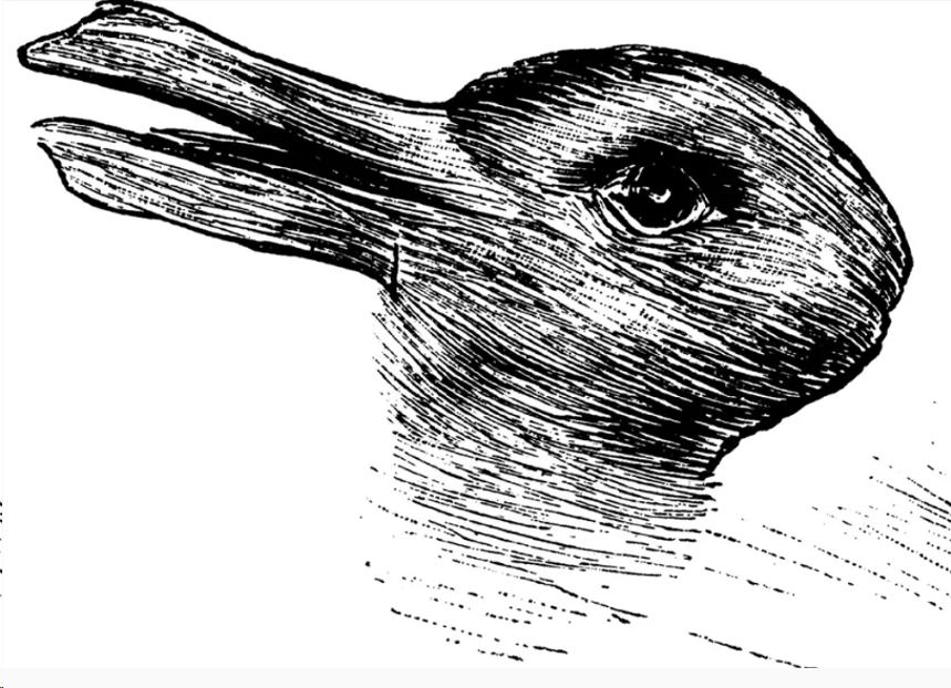
This is a well known optical illusion, which first appeared in a German humor magazine back in 1892. As you could notice, you can see either duck or rabbit, depending on how you observe the image. What is happening in this and similar illusions is that they use previously mentioned functions of the visual cortex to confuse us. Take a look at the same image bellow:

If your attention wanders to the area where the red square is you would say that you see a duck. However, if you are focused on the area of the image marked with a blue square, you would say that you see a rabbit.
Meaning, when you observe certain features of the image different group of neurons got activated and you classify this image either like a rabbit or like a duck. This is exactly the functionality that Convolutional Neural Networks utilize. They detect features on the image and then classify them based on that inforamtion.

We will not go into details of how
Than Convolutional Neural Network use additional layers to remove linearity from the image, something that could cause overfitting. When linearity is removed, additional layers for compressing the image (polling) and flattening the data are used.
Finally, this information is passed into a neural network, called Fully-Connected Layer in the world of Convolutional Neural Networks. Again, the goal of this article is to show you how to implement all these concepts, so more details about these layers, how they work and what is the purpose of each of them can be found here.

3. Dataset and Installation of Tensorflow.js
3.1 Dataset
In one of the previous articles, we implemented this type of neural networks using Python and Keras. We created a neural network that is able to detect and classify handwritten digits. For that purpose, we used MNIST dataset.
This is a well-known dataset in the world of neural networks. It is extending its predecessor NIST and it has a training set of 60,000 samples and testing set of 10,000 images of handwritten digits. All digits have been size-normalized and centered. Size of the images is also fixed to 28×28 pixels. This is why this dataset is so popular.

Using Convolutional Neural Networks we can get almost human results. The record, when it comes to accuracy of prediction on this dataset, is held by the Parallel Computing Center (Khmelnitskiy, Ukraine). They used an ensemble of only 5 convolution neural networks and got the error rate of 0.21 percent. Basically, they are giving correct results in 99.79% of the cases. Awesome, isn’t it?
For the implementation in JavaScript that we plan to do here we will also need a simple HTTP server. I am using this one, which can be easily installed using
> npm install http-server
It is run using command:
> http-server
3.2 Installing Tensorflow.js
There are several ways in which we can use TensorFlow.js. First one, of course, is using it just by adding script tag inside of our main HTML file:
<script src="https://cdn.jsdelivr.net/npm/@tensorflow/tfjs@1.0.0/dist/tf.min.js"></script>
You can also install it using npm or yarn for setting it up under Node.js:
npm install @tensorflow/tfjs
yarn add @tensorflow/tfjs
4. Loading Data
In order to faster load fore-mentioned data, guys from Google provided us with this sprite file and with this code so we can manage that sprite file. However, I had to tweak this code a little bit to better fit my needs, so here how it looks like:
const IMAGE_SIZE = 784;
const NUM_CLASSES = 10;
const NUM_DATASET_ELEMENTS = 65000;

const TRAIN_TEST_RATIO = 5 / 6;

const NUM_TRAIN_ELEMENTS = Math.floor(TRAIN_TEST_RATIO * NUM_DATASET_ELEMENTS);
const NUM_TEST_ELEMENTS = NUM_DATASET_ELEMENTS - NUM_TRAIN_ELEMENTS;

const MNIST_IMAGES_SPRITE_PATH =
    'https://storage.googleapis.com/learnjs-data/model-builder/mnist_images.png';
const MNIST_LABELS_PATH =
    'https://storage.googleapis.com/learnjs-data/model-builder/mnist_labels_uint8';

/**
 * A class that fetches the sprited MNIST dataset and returns shuffled batches.
 *
 * NOTE: This will get much easier. For now, we do data fetching and
 * manipulation manually.
 */
export class MnistData {
  constructor() {
    this.shuffledTrainIndex = 0;
    this.shuffledTestIndex = 0;
  }

  async load() {
    // Make a request for the MNIST sprited image.
    const img = new Image();
    const canvas = document.createElement('canvas');
    const ctx = canvas.getContext('2d');
    const imgRequest = new Promise((resolve, reject) => {
      img.crossOrigin = '';
      img.onload = () => {
        img.width = img.naturalWidth;
        img.height = img.naturalHeight;

        const datasetBytesBuffer =
            new ArrayBuffer(NUM_DATASET_ELEMENTS * IMAGE_SIZE * 4);

        const chunkSize = 5000;
        canvas.width = img.width;
        canvas.height = chunkSize;

        for (let i = 0; i < NUM_DATASET_ELEMENTS / chunkSize; i++) {
          const datasetBytesView = new Float32Array(
              datasetBytesBuffer, i * IMAGE_SIZE * chunkSize * 4,
              IMAGE_SIZE * chunkSize);
          ctx.drawImage(
              img, 0, i * chunkSize, img.width, chunkSize, 0, 0, img.width,
              chunkSize);

          const imageData = ctx.getImageData(0, 0, canvas.width, canvas.height);

          for (let j = 0; j < imageData.data.length / 4; j++) {
            // All channels hold an equal value since the image is grayscale, so
            // just read the red channel.
            datasetBytesView[j] = imageData.data[j * 4] / 255;
          }
        }
        this.datasetImages = new Float32Array(datasetBytesBuffer);

        resolve();
      };
      img.src = MNIST_IMAGES_SPRITE_PATH;
    });

    const labelsRequest = fetch(MNIST_LABELS_PATH);
    const [imgResponse, labelsResponse] =
        await Promise.all([imgRequest, labelsRequest]);

    this.datasetLabels = new Uint8Array(await labelsResponse.arrayBuffer());

    // Create shuffled indices into the train/test set for when we select a
    // random dataset element for training / validation.
    this.trainIndices = tf.util.createShuffledIndices(NUM_TRAIN_ELEMENTS);
    this.testIndices = tf.util.createShuffledIndices(NUM_TEST_ELEMENTS);

    // Slice the the images and labels into train and test sets.
    this.trainImages =
        this.datasetImages.slice(0, IMAGE_SIZE * NUM_TRAIN_ELEMENTS);
    this.testImages = this.datasetImages.slice(IMAGE_SIZE * NUM_TRAIN_ELEMENTS);
    this.trainLabels =
        this.datasetLabels.slice(0, NUM_CLASSES * NUM_TRAIN_ELEMENTS);
    this.testLabels =
        this.datasetLabels.slice(NUM_CLASSES * NUM_TRAIN_ELEMENTS);
  }

  nextDataBatch(batchSize, test = false) {
    if(test)
        return this.nextBatch(
            batchSize, [this.trainImages, this.trainLabels], () => {
              this.shuffledTrainIndex =
                  (this.shuffledTrainIndex + 1) % this.trainIndices.length;
              return this.trainIndices[this.shuffledTrainIndex];
            });
    else
        return this.nextBatch(batchSize, [this.testImages, this.testLabels], () => {
            this.shuffledTestIndex =
                (this.shuffledTestIndex + 1) % this.testIndices.length;
            return this.testIndices[this.shuffledTestIndex];
          });
  }

  nextBatch(batchSize, data, index) {
    const batchImagesArray = new Float32Array(batchSize * IMAGE_SIZE);
    const batchLabelsArray = new Uint8Array(batchSize * NUM_CLASSES);

    for (let i = 0; i < batchSize; i++) {
      const idx = index();

      const image =
          data[0].slice(idx * IMAGE_SIZE, idx * IMAGE_SIZE + IMAGE_SIZE);
      batchImagesArray.set(image, i * IMAGE_SIZE);

      const label =
          data[1].slice(idx * NUM_CLASSES, idx * NUM_CLASSES + NUM_CLASSES);
      batchLabelsArray.set(label, i * NUM_CLASSES);
    }

    const xs = tf.tensor2d(batchImagesArray, [batchSize, IMAGE_SIZE]);
    const labels = tf.tensor2d(batchLabelsArray, [batchSize, NUM_CLASSES]);

    return {xs, labels};
  }
}
Here are some major points of this MnistData class. Images and labels of those images are loaded into fields trainImages,
5. Implementation of Image Classifcation with Tensorflow.js
Let’s start from index.html file of our solution. In the previous article, we presented several ways of installing TensorFlow.js. One of them was integrating it within script tag of the HTML file. That is what is done here:
<!DOCTYPE html>
<html>
<head>
  <meta charset="utf-8">
  <meta http-equiv="X-UA-Compatible" content="IE=edge">
  <meta name="viewport" content="width=device-width, initial-scale=1.0">
  <title>TensorFlow.js Convolutional Neural Networks</title>
  <script src="https://cdn.jsdelivr.net/npm/@tensorflow/tfjs@1.0.0/dist/tf.min.js"></script>
  <script src="https://cdn.jsdelivr.net/npm/@tensorflow/tfjs-vis@1.0.2/dist/tfjs-vis.umd.min.js"></script>
  <script src="./data.js" type="module"></script>
  <script src="./script.js" type="module"></script>
</head>

<body>
</body>
</html>
Note that we add the script tag for TensorFlow.js and additional for
Now, let’s examine the script.js file, where the
async function run() {
    const data = await getData();

    await displayDataFunction(data, 30);

    const model = createModel();
    tfvis.show.modelSummary({name: 'Model Architecture'}, model);

    await trainModel(model, data, 20);

    await evaluateModel(model, data);
}
You can notice that this function is similar to the one from the previous article. It reveals the workflow of the application. In the beginning, we load the data using
async function getDataFunction() {
    var data = new MnistData();
    await data.load();
    return data;
}
First, we create an object of MnistData class. This class is located in
async function singleImagePlot(image)
{
  const canvas = document.createElement('canvas');
  canvas.width = 28;
  canvas.height = 28;
  canvas.style = 'margin: 4px;';
  await tf.browser.toPixels(image, canvas);
  return canvas;
}

async function displayDataFunction(data, numOfImages = 10) {

  const inputDataSurface =
    tfvis.visor().surface({ name: 'Input Data Examples', tab: 'Input Data'});

  const examples = data.nextDataBatch(numOfImages, true);

  for (let i = 0; i < numOfImages; i++) {
    const image = tf.tidy(() => {
      return examples.xs
        .slice([i, 0], [1, examples.xs.shape[1]])
        .reshape([28, 28, 1]);
    });

    const canvas = await singleImagePlot(image)
    inputDataSurface.drawArea.appendChild(canvas);

    image.dispose();
  }
}
In this function, we first create a new tab called Input Data. Then we get a batch of test data using

Once data is visualized, we can proceed to the more fun part of the
function createModelFunction() {
  const cnn = tf.sequential();

  cnn.add(tf.layers.conv2d({
      inputShape: [28, 28, 1],
      kernelSize: 5,
      filters: 8,
      strides: 1,
      activation: 'relu',
      kernelInitializer: 'varianceScaling'
    }));
  cnn.add(tf.layers.maxPooling2d({poolSize: [2, 2], strides: [2, 2]}));

  cnn.add(tf.layers.conv2d({
      kernelSize: 5,
      filters: 16,
      strides: 1,
      activation: 'relu',
      kernelInitializer: 'varianceScaling'
    }));
  cnn.add(tf.layers.maxPooling2d({poolSize: [2, 2], strides: [2, 2]}));

  cnn.add(tf.layers.flatten());

  cnn.add(tf.layers.dense({
    units: 10,
    kernelInitializer: 'varianceScaling',
    activation: 'softmax'
  }));

  cnn.compile({
    optimizer: tf.train.adam(),
    loss: 'categoricalCrossentropy',
    metrics: ['accuracy'],
  });

  return cnn;
}
Basically, we create two convolutional layers that are followed by max-polling layers. Finally, we flatten the data into an array and put it through a fully connected layer, which is in this case just one dense layer with 10 neurons. This last layer is actually the output layer, which predicts the class of the image. Model is then compiled with categorical cross-entropy and Adam optimizer. Once we print the summary of the model with

Cool! Now, we have prepared input data and model, so we can train it. This is done inside trainModel function:
async function trainModelFunction(model, data, epochs) {
    const metrics = ['loss', 'val_loss', 'acc', 'val_acc'];
    const container = {
      name: 'Model Training', styles: { height: '1000px' }
    };
    const fitCallbacks = tfvis.show.fitCallbacks(container, metrics);

    const batchSize = 512;

    const [trainX, trainY] = getBatch(data, 5500);
    const [testX, testY] = getBatch(data, 1000, true);

    return model.fit(trainX, trainY, {
      batchSize: batchSize,
      validationData: [testX, testY],
      epochs: epochs,
      shuffle: true,
      callbacks: fitCallbacks
    });
}
In essence, we get a batch of train data and a batch of test data. Then we ignite fit method on our model and pass the train data for training and test data for evaluation. Metrics like loss and accuracy are displayed after each epoch using

The final step in this process if the evaluation of our model. For that purpose, we display accuracy per digit and we use the concept of a confusion matrix. This matrix is just a table that is often used to describe the performance of a classification model. This all is done in the
function predict(model, data, testDataSize = 500) {
  const testData = data.nextDataBatch(testDataSize, true);
  const testxs = testData.xs.reshape([testDataSize, 28, 28, 1]);
  const labels = testData.labels.argMax([-1]);
  const preds = model.predict(testxs).argMax([-1]);

  testxs.dispose();
  return [preds, labels];
}

async function displayAccuracyPerClass(model, data) {
  const [preds, labels] = predict(model, data);
  const classAccuracy = await tfvis.metrics.perClassAccuracy(labels, preds);
  const container = {name: 'Accuracy', tab: 'Evaluation'};
  tfvis.show.perClassAccuracy(container, classAccuracy, classNames);

  labels.dispose();
}

async function displayConfusionMatrix(model, data) {
  const [preds, labels] = predict(model, data);
  const confusionMatrix = await tfvis.metrics.confusionMatrix(labels, preds);
  const container = {name: 'Confusion Matrix', tab: 'Evaluation'};
  tfvis.render.confusionMatrix(
      container, {values: confusionMatrix}, classNames);

  labels.dispose();
}

async function evaluateModelFunction(model, data)
{
  await displayAccuracyPerClass(model, data);
  await displayConfusionMatrix(model, data);
}
As you can see, this function is using helper functions like displayAccuracyPerClass, displayConfusionMatrix and predict to make thise graphs:

We are getting pretty good results with this simple model and with just 20 epochs. We could improve these results by adding additional convolutional layers or increasing number of epochs. This would, of course, get an impact on the length of the training process.
Conclusion
In this article, we got a chance to see how we can utilize Convolutional Neural Networks with TensorFlow.js. We learned how to manipulate layers that are specific for this type of neural networks and run them inside of a browser.
Thank you for reading!
This bundle of e-books is specially crafted for beginners.
Everything from Python basics to the deployment of Machine Learning algorithms to production in one place.
Become a Machine Learning Superhero TODAY!

Nikola M. Zivkovic
CAIO at Rubik's Code
Nikola M. Zivkovic is the author of books: Ultimate Guide to Machine Learning and Deep Learning for Programmers. He loves knowledge sharing, and he is an experienced speaker. You can find him speaking at meetups, conferences, and as a guest lecturer at the University of Novi Sad.


Trackbacks/Pingbacks