Why Training a Neural Network Is Hard

Or, Why Stochastic Gradient Descent Is Used to Train Neural Networks.

Fitting a neural network involves using a training dataset to update the model weights to create a good mapping of inputs to outputs.

This training process is solved using an optimization algorithm that searches through a space of possible values for the neural network model weights for a set of weights that results in good performance on the training dataset.

In this post, you will discover the challenge of training a neural network framed as an optimization problem.

After reading this post, you will know:

• Training a neural network involves using an optimization algorithm to find a set of weights to best map inputs to outputs.
• The problem is hard, not least because the error surface is non-convex and contains local minima, flat spots, and is highly multidimensional.
• The stochastic gradient descent algorithm is the best general algorithm to address this challenging problem.

Kick-start your project with my new book Better Deep Learning, including step-by-step tutorials and the Python source code files for all examples.

Let’s get started.

Why Training a Neural Network Is Hard
Photo by Loren Kerns, some rights reserved.

Overview

This tutorial is divided into four parts; they are:

1. Learning as Optimization
2. Challenging Optimization
3. Features of the Error Surface
4. Implications for Training

Learning as Optimization

Deep learning neural network models learn to map inputs to outputs given a training dataset of examples.

The training process involves finding a set of weights in the network that proves to be good, or good enough, at solving the specific problem.

This training process is iterative, meaning that it progresses step by step with small updates to the model weights each iteration and, in turn, a change in the performance of the model each iteration.

The iterative training process of neural networks solves an optimization problem that finds for parameters (model weights) that result in a minimum error or loss when evaluating the examples in the training dataset.

Optimization is a directed search procedure and the optimization problem that we wish to solve when training a neural network model is very challenging.

This raises the question as to what exactly is so challenging about this optimization problem?

Challenging Optimization

Training deep learning neural networks is very challenging.

The best general algorithm known for solving this problem is stochastic gradient descent, where model weights are updated each iteration using the backpropagation of error algorithm.

Optimization in general is an extremely difficult task. […] When training neural networks, we must confront the general non-convex case.

— Page 282, Deep Learning, 2016.

An optimization process can be understood conceptually as a search through a landscape for a candidate solution that is sufficiently satisfactory.

A point on the landscape is a specific set of weights for the model, and the elevation of that point is an evaluation of the set of weights, where valleys represent good models with small values of loss.

This is a common conceptualization of optimization problems and the landscape is referred to as an “error surface.”

In general, E(w) [the error function of the weights] is a multidimensional function and impossible to visualize. If it could be plotted as a function of w [the weights], however, E [the error function] might look like a landscape with hills and valleys …

— Page 113, Neural Smithing: Supervised Learning in Feedforward Artificial Neural Networks, 1999.

The optimization algorithm iteratively steps across this landscape, updating the weights and seeking out good or low elevation areas.

For simple optimization problems, the shape of the landscape is a big bowl and finding the bottom is easy, so easy that very efficient algorithms can be designed to find the best solution.

These types of optimization problems are referred to mathematically as convex.

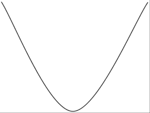
Example of a Convex Error Surface

The error surface we wish to navigate when optimizing the weights of a neural network is not a bowl shape. It is a landscape with many hills and valleys.

These type of optimization problems are referred to mathematically as non-convex.

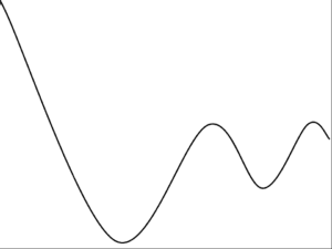
Example of a Non-Convex Error Surface

In fact, there does not exist an algorithm to solve the problem of finding an optimal set of weights for a neural network in polynomial time. Mathematically, the optimization problem solved by training a neural network is referred to as NP-complete (e.g. they are very hard to solve).

We prove this problem NP-complete and thus demonstrate that learning in neural networks has no efficient general solution.

— Neural Network Design and the Complexity of Learning, 1988.

Key Features of the Error Surface

There are many types of non-convex optimization problems, but the specific type of problem we are solving when training a neural network is particularly challenging.

We can characterize the difficulty in terms of the features of the landscape or error surface that the optimization algorithm may encounter and must navigate in order to be able to deliver a good solution.

There are many aspects of the optimization of neural network weights that make the problem challenging, but three often-mentioned features of the error landscape are the presence of local minima, flat regions, and the high-dimensionality of the search space.

Backpropagation can be very slow particularly for multilayered networks where the cost surface is typically non-quadratic, non-convex, and high dimensional with many local minima and/or flat regions.

— Page 13, Neural Networks: Tricks of the Trade, 2012.

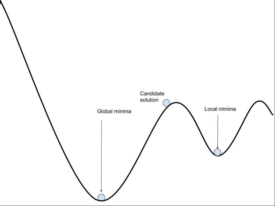
1. Local Minima

Local minimal or local optima refer to the fact that the error landscape contains multiple regions where the loss is relatively low.

These are valleys, where solutions in those valleys look good relative to the slopes and peaks around them. The problem is, in the broader view of the entire landscape, the valley has a relatively high elevation and better solutions may exist.

It is hard to know whether the optimization algorithm is in a valley or not, therefore, it is good practice to start the optimization process with a lot of noise, allowing the landscape to be sampled widely before selecting a valley to fall into.

By contrast, the lowest point in the landscape is referred to as the “global minima“.

Neural networks may have one or more global minima, and the challenge is that the difference between the local and global minima may not make a lot of difference.

The implication of this is that often finding a “good enough” set of weights is more tractable and, in turn, more desirable than finding a global optimal or best set of weights.

Nonlinear networks usually have multiple local minima of differing depths. The goal of training is to locate one of these minima.

— Page 14, Neural Networks: Tricks of the Trade, 2012.

A classical approach to addressing the problem of local minima is to restart the search process multiple times with a different starting point (random initial weights) and allow the optimization algorithm to find a different, and hopefully better, local minima. This is called “multiple restarts”.

Random Restarts: One of the simplest ways to deal with local minima is to train many different networks with different initial weights.

— Page 121, Neural Smithing: Supervised Learning in Feedforward Artificial Neural Networks, 1999.

2. Flat Regions (Saddle Points)

A flat region or saddle point is a point on the landscape where the gradient is zero.

These are flat regions at the bottom of valleys or regions between peaks. The problem is that a zero gradient means that the optimization algorithm does not know which direction to move in order to improve the model.

… the presence of saddlepoints, or regions where the error function is very flat, can cause some iterative algorithms to become ‘stuck’ for extensive periods of time, thereby mimicking local minima.

— Page 255, Neural Networks for Pattern Recognition, 1995.

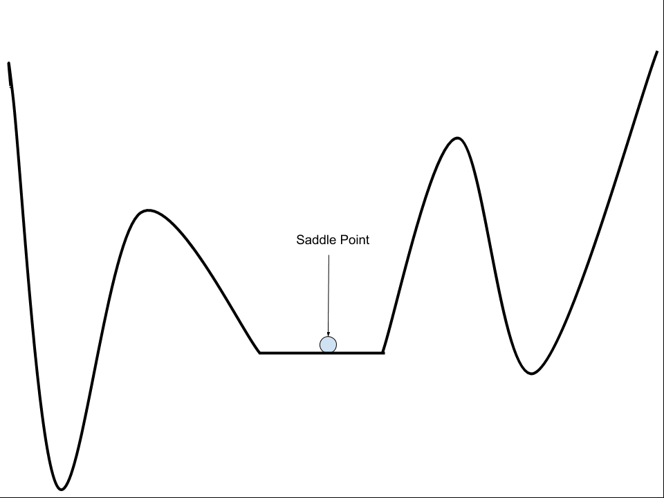
Example of a Saddlepoint on an Error Surface

Nevertheless, recent work may suggest that perhaps local minima and flat regions may be less of a challenge than was previously believed.

Do neural networks enter and escape a series of local minima? Do they move at varying speed as they approach and then pass a variety of saddle points? […] we present evidence strongly suggesting that the answer to all of these questions is no.

— Qualitatively characterizing neural network optimization problems, 2015.

3. High-Dimensional

The optimization problem solved when training a neural network is high-dimensional.

Each weight in the network represents another parameter or dimension of the error surface. Deep neural networks often have millions of parameters, making the landscape to be navigated by the algorithm extremely high-dimensional, as compared to more traditional machine learning algorithms.

The problem of navigating a high-dimensional space is that the addition of each new dimension dramatically increases the distance between points in the space, or hypervolume. This is often referred to as the “curse of dimensionality”.

This phenomenon is known as the curse of dimensionality. Of particular concern is that the number of possible distinct configurations of a set of variables increases exponentially as the number of variables increases.

— Page 155, Deep Learning, 2016.

Implications for Training

The challenging nature of optimization problems to be solved when using deep learning neural networks has implications when training models in practice.

In general, stochastic gradient descent is the best algorithm available, and this algorithm makes no guarantees.

There is no formula to guarantee that (1) the network will converge to a good solution, (2) convergence is swift, or (3) convergence even occurs at all.

— Page 13, Neural Networks: Tricks of the Trade, 2012.

We can summarize these implications as follows:

• Possibly Questionable Solution Quality. The optimization process may or may not find a good solution and solutions can only be compared relatively, due to deceptive local minima.
• Possibly Long Training Time. The optimization process may take a long time to find a satisfactory solution, due to the iterative nature of the search.
• Possible Failure. The optimization process may fail to progress (get stuck) or fail to locate a viable solution, due to the presence of flat regions.

The task of effective training is to carefully configure, test, and tune the hyperparameters of the model and the learning process itself to best address this challenge.

Thankfully, modern advancements can dramatically simplify the search space and accelerate the search process, often discovering models much larger, deeper, and with better performance than previously thought possible.

Further Reading

This section provides more resources on the topic if you are looking to go deeper.

Books

• Deep Learning, 2016.
• Neural Networks: Tricks of the Trade, 2012.
• Neural Networks for Pattern Recognition, 1995.
• Neural Smithing: Supervised Learning in Feedforward Artificial Neural Networks, 1999.

Papers

• Training a 3-Node Neural Network is NP-Complete, 1992.
• Qualitatively characterizing neural network optimization problems, 2015.
• Neural Network Design and the Complexity of Learning, 1988.

Articles

• The hard thing about deep learning, 2016.
• Saddle point, Wikipedia.
• Curse of dimensionality, Wikipedia.
• NP-completeness, Wikipedia.

Summary

In this post, you discovered the challenge of training a neural network framed as an optimization problem.

Specifically, you learned:

• Training a neural network involves using an optimization algorithm to find a set of weights to best map inputs to outputs.
• The problem is hard, not least because the error surface is non-convex and contains local minima, flat spots, and is highly multidimensional.
• The stochastic gradient descent algorithm is the best general algorithm to address this challenging problem.

Do you have any questions?
Ask your questions in the comments below and I will do my best to answer.

Develop Better Deep Learning Models Today!

Train Faster, Reduce Overftting, and Ensembles

...with just a few lines of python code

Discover how in my new Ebook:
Better Deep Learning

It provides self-study tutorials on topics like:
weight decay, batch normalization, dropout, model stacking and much more...

Bring better deep learning to your projects!

Skip the Academics. Just Results.

See What's Inside