

Check out new guide with ML 1.0 here.
Code that accompanies this article can be downloaded here.
Several months ago I wrote a series of articles about ML.NET. Back then ML.NET was at its infancy and I used 0.3 version to solve some real-world problems. One of my examples even ended up in the official ML.NET GitHub. However, guys at Microsoft decided to change the whole ML.NET API in version 0.6 making my articles somewhat outdated. Apart from that, we had two previews of .NET Core 3 in the last two months, which means it will be out soon-ish.

ML.NET should be a part of .NET Core 3 release, so my assumption is that there won’t be any ground-breaking changes in the API once again. This is why I decided to write another article on this topic and cover all the things once again, but using the new API. To be honest, changing from 0.3 ML.NET version to 0.10 ML.NET version (latest version) were not as straight-forward as I hoped so. Some of the things I don’t like so much, others I adored. So, buckle up, this is going to be a wild ride.
Why Machine Learning?

Before we dive into the problems ahead of us, let’s take a moment and reflect why is Microsoft introducing this technology and why should we consider studying machine learning today. Well, there are several reasons for that. First one is that the technology is crossing the chasm. We are moving from the period where this was some obscure science that only a few practiced and understood to a place where it is a norm. Today we can build our own machine learning models that could solve real at our own home. Python and R became leading languages in this area and they already have a wide range of libraries. Microsoft didn’t provided us with these options thus far apart from Azure Machine Learning for cloud-based analytics.

The other reason why you should consider exploring machine learning, deep learning, and data science is the fact that we are producing a lot of data. We as humans are not able to process that data and make the science of it, but machine learning models can. The statistics say that from the beginning of time up until 2005. humans have produced 130 Exabytes of data. Exabyte is a real word, by the way, I checked it 🙂 Basically, if you scale up from terabyte you get petabyte and when you scale from petabyte you get exabyte.
What is interesting is that from that moment up until 2010. we produced 1200 exabytes of data, and until 2015. we produced 7900 exabytes of data. Predictions for the future are telling us that there will be only more and more data and that 2025. we will have 193 Zettabytes of data, which is one level above Exabyte. In a nutshell, we are having more and more data, and more and more practical use of it.
Another interesting fact is that the ideas behind machine learning are going long back. You can observe it as this weird steampunk science because the concepts we use and explore today are based on some “ancient” knowledge. Byes theorem was presended in 1763, and Markov’s chains in 1913. The idea of a learning machine can be traced back to the 50s, to the Turing’s Learning Machine and Frank Rosenbllat’s Perceptron. This means that we have 50+ years of knowledge to back us up. To sum it up, we are at a specific point in history, where we have a lot of knowledge, we have a lot of data and we have the technology. So it is up to us to use those tools as best as we can.
What is Machine Learning?

Machine Learning is considered to be a sub-branch of artificial intelligence, and it uses statistical techniques to give computers the ability to learn how to solve certain problems, instead of explicitly programming it. As mentioned, all important machine learning concepts can be traced back to the 1950s. The main idea, however, is to develop a mathematical model which will be able to make some predictions. This model is usually trained on some data beforehand.
In a nutshell, the mathematical model uses insights made on old data to make predictions on new data. This whole process is called predictive modeling. If we put it mathematically we are trying to approximate a mapping function – f from input variables X to output variables y. There are two big groups of problems we are trying to solve using this approach: Regression and Classification.
Regression problems require prediction of the quantity. This means our output is continuous, real-value, usually an integer or floating point value. For example, we want to predict the price of the company shares based on the data from the past couple of months. Classification problems are a bit different. They are trying to divide an input into certain categories. This means that the output of this tasks is discrete. For example, we are trying to predict the class of fruit on its dimensions. In this article, we will consider one real-world problem from both groups of problems and solve them with ML.NET.
Building a Machine Learning Model

In general, there are several steps we can follow when we are building a machine learning model. Here there are:
- Data Analysis
- Applying Proper Algorithm
- Evaluation
At the moment, ML.NET is not giving us too many options when it comes to the Data Analysis area, so in these examples, I will use Python to get information that I need. This is probably the only thing that I don’t like about
- Univariate Analysis – Analysing types and nature of every feature.
- Missing Data Treatment – Detecting missing data and making a strategy about it.
- Outlier Detection – Detecting anomalies in the data. Outliers are samples that diverge from an overall pattern in some data.
- Correlation Analysis – Comparing features among each other.
Using information from this analysis we can take appropriate actions during the model creation. ML.NET is giving us a lot of precooked algorithms and means to use them quickly. Also, it is easy to tune each of these mechanisms. In this article, I will try to use as many algorithms as possible, but I will not go in depth and explain them in details. Another note is that I will use only the default setups of these algorithms. Take into consideration that you can get better results if you tune them up differently.
Installing ML.NET

If you want to use ML.NET in your project, you need to have at least .NET Core 2.0, so make sure you have it installed on your computer. The other thing you should know is that it currently must run in the 64-bit process. Keep this in mind while making your .NET Core project. Installation is pretty straight forward with
Install-Package Microsoft.ML -version 0.2+10
This can be achieved by sing .NET Core CLI. If you are going to do it this way, make sure you have installed .NET Core SDK and run this command:
dotnet add package Microsoft.ML --version 0.10.0
Alternatively, you can use Visual Studio’s Manage NuGetPackage option:

After that, search for Microsoft.ML and install it.
Regression Problem – Bike Share Demand

Bike sharing systems work like rent-a-car systems, but for bikes. Basically, a number of locations in the city are provided where the whole process of obtaining a membership, renting a bicycle and returning it is automated. Users can rent a bicycle in one location and return it to a different location. There are more than 500 cities around the world with these systems at the moment.
The cool thing about these systems, apart from being good for the environment, is that they record everything that is happening. When this data is combined with weather data, we can use it for investigating many topics, like pollution and traffic mobility. That is exactly what we have on our hands in Bike Sharing Demands Dataset. This dataset is provided by the Capital Bikeshare program from Washington, D.C.
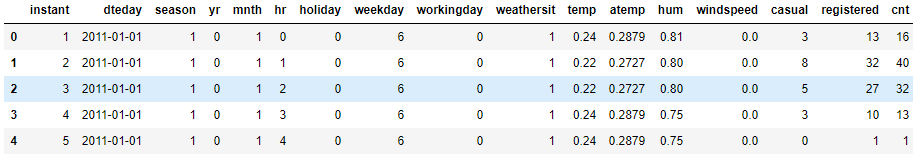
This dataset has two files, one for the hourly (hour.csv) records
In this article, we will use only hourly samples. Here is how that looks:

The hour.csv file contains following features (attributes):
- Instant – sample index
- Dteday – Date when the sample was recorded
- Season – Season in which sample was recorded
- Spring – 1
- Summer – 2
- Fall – 3
- Winter – 4
- Yr – Year in which sample was recorded
- The year 2011 – 0
- The year 2012 – 1
- Mnth – Month in which sample was recorded
- Hr – Hour in which sample was recorded
- Holiday – Weather day is a holiday or not (extracted from [Web Link])
- Weekday – Day of the week
- Workingday – If the day is neither weekend nor holiday is 1, otherwise is 0.
- Weathersit – Kind of weather that was that day when the sample was recorded
- Clear, Few clouds, Partly cloudy, Partly cloudy – 1
- Mist + Cloudy, Mist + Broken clouds, Mist + Few clouds, Mist – 2
- Light Snow, Light Rain + Thunderstorm + Scattered clouds, Light Rain + Scattered clouds – 3
- Heavy Rain + Ice Pallets + Thunderstorm + Mist, Snow + Fog – 4
- Temp – Normalized temperature in Celsius.
- Atemp – Normalized feeling temperature in Celsius.
- Hum – Normalized humidity.
- Windspeed – Normalized wind speed.
- Casual – Count of casual users
- Registered – Count of registered users
- Cnt – Count of total rental bikes including both casual and registered
Data Analysis
From first glance at the data, we can see that we are having some features that are categorical (Season, Hour, Holiday, Weather…). To put it simply, this means that some data behaves as an enumeration. It is an important fact for our mathematical model and we need to handle it during model creation. Another thing that we can notice is that some features are not on the same scale. This is something we should consider as well. We got both of these facts from univariate analysis, ie. observing nature of every feature:
During the next step, the Missing Data Treatment step, we haven’t detected any missing data in any of the features:

Next, we have performed an outlier analysis. Using Python, we are able to plot the distribution of data, so during this analysis that is exactly what we do. We observe the distribution of certain features and detect samples with values that are far off. Let’s observe two distributions, Count distribution and Hour/Count distribution:

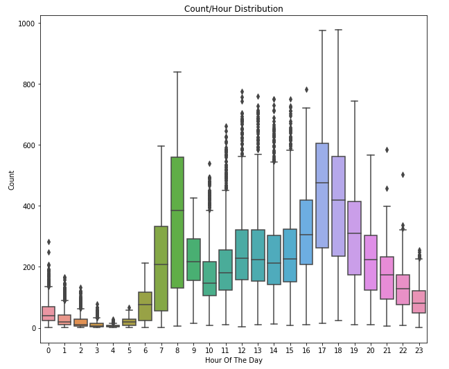
Note the dots that the red arrow points to in the first picture. These are outliers, ie. values that are out of general distribution which is represented with a blue rectangle. There are quite a lot of them. Samples with these values are introducing a non-linearity in our system. We may choose to remove them from the dataset or keep them if we want to avoid linearity. For the purpose of this article, we are going to keep them. On the second image, we can see that most of the bikes are rented at the beginning of working hours and at the end of it.
Finally, we performed some correlation analysis. During this step we are checking is there any connection between features in the dataset. Using Python we were able to get this image which shows matrix with levels of dependency between some of the features – correlation matrix:

We wanted to find the relationship between count and some of the features using this correlation matrix. The values, as you can see, are between -1 and
1. We are aiming for the ones that have a value close to 1, which means that these features have too much in common, ie. too much influence on each other. If we have that situation it is suggested to provide just one of those features to a machine learning model.
This way we would avoid the situation in which our machine learning model gives overly optimistic (or plain wrong) predictions. From the matrix above, we can see that
Implementation
Ok, we are finally here. The solution we are going to present here is not just creating one machine learning model. We are going run several regression algorithms from ML.NET on this dataset and evaluate which one worked the best. The whole code that accompanies this article can be found here.
Handling Data
There is one technicality that needs to be done before implementing the solution. The usual practice is to divide the presented dataset into a training set and testing set. This way we can evaluate our model without fear that it is biased. Another usual practice is that 80% of data goes into the training set and 20% to the testing set. However, you can use different ratio if it better suites your data.
Here is how one of these files look like:

Once we separated data into these sets we need to create classes that can handle them. Two classes: BikeSharingDemandSample and BikeSharingDemandPrediction located in BikeSharingDemandData folder are used for that. Objects of these classes will handle information from .csv files. Take a look at the way they are implemented:
| using Microsoft.ML.Data; | |
| namespace BikeSharingDemand.BikeSharingDemandData | |
| { | |
| public class BikeSharingDemandSample | |
| { | |
| [Column("2")] public float Season; | |
| [Column("3")] public float Year; | |
| [Column("4")] public float Month; | |
| [Column("5")] public float Hour; | |
| [Column("6")] public bool Holiday; | |
| [Column("7")] public float Weekday; | |
| [Column("8")] public float Weather; | |
| [Column("9")] public float Temperature; | |
| [Column("10")] public float NormalizedTemperature; | |
| [Column("11")] public float Humidity; | |
| [Column("12")] public float Windspeed; | |
| [Column("16")] public float Count; | |
| } | |
| public class BikeSharingDemandPrediction | |
| { | |
| [ColumnName("Score")] | |
| public float PredictedCount; | |
| } | |
| } | |
The important thing to notice is that some features are not on the list, ie. we skipped some of the columns from the dataset. This is done based on data analysis that we previously have done. We removed the
Building the Model
The whole process of creating a model and generating predictions is located inside of the Model class. This class is used as a wrapper for all the operations we want to perform. Here is how it looks like:
| using BikeSharingDemand.BikeSharingDemandData; | |
| using Microsoft.Data.DataView; | |
| using Microsoft.ML; | |
| using Microsoft.ML.Core.Data; | |
| using Microsoft.ML.Data; | |
| using Microsoft.ML.Training; | |
| using System.IO; | |
| using System.Linq; | |
| namespace BikeSharingDemand.ModelNamespace | |
| { | |
| public sealed class Model | |
| { | |
| private readonly MLContext _mlContext; | |
| private PredictionEngine<BikeSharingDemandSample, BikeSharingDemandPrediction> _predictionEngine; | |
| private ITransformer _trainedModel; | |
| private TextLoader _textLoader; | |
| private ITrainerEstimator<ISingleFeaturePredictionTransformer<IPredictor>, IPredictor> _algorythim; | |
| public string Name { get; private set; } | |
| public Model(MLContext mlContext, ITrainerEstimator<ISingleFeaturePredictionTransformer<IPredictor>, IPredictor> algorythm) | |
| { | |
| _mlContext = mlContext; | |
| _algorythim = algorythm; | |
| _textLoader = _mlContext.Data.CreateTextLoader(new TextLoader.Arguments() | |
| { | |
| Separators = new[] { ',' }, | |
| HasHeader = true, | |
| Column = new[] | |
| { | |
| new TextLoader.Column("Season", DataKind.R4, 2), | |
| new TextLoader.Column("Year", DataKind.R4, 3), | |
| new TextLoader.Column("Month", DataKind.R4, 4), | |
| new TextLoader.Column("Hour", DataKind.R4, 5), | |
| new TextLoader.Column("Holiday", DataKind.Bool, 6), | |
| new TextLoader.Column("Weekday", DataKind.R4, 7), | |
| new TextLoader.Column("Weather", DataKind.R4, 8), | |
| new TextLoader.Column("Temperature", DataKind.R4, 9), | |
| new TextLoader.Column("NormalizedTemperature", DataKind.R4, 10), | |
| new TextLoader.Column("Humidity", DataKind.R4, 11), | |
| new TextLoader.Column("Windspeed", DataKind.R4, 12), | |
| new TextLoader.Column("Count", DataKind.R4, 16), | |
| } | |
| }); | |
| Name = algorythm.GetType().ToString().Split('.').Last(); | |
| } | |
| public void BuildAndFit(string trainingDataViewLocation) | |
| { | |
| IDataView trainingDataView = _textLoader.Read(trainingDataViewLocation); | |
| var pipeline = _mlContext.Transforms.CopyColumns(inputColumnName: "Count", outputColumnName: "Label") | |
| .Append(_mlContext.Transforms.Categorical.OneHotEncoding("Season")) | |
| .Append(_mlContext.Transforms.Categorical.OneHotEncoding("Year")) | |
| .Append(_mlContext.Transforms.Categorical.OneHotEncoding("Month")) | |
| .Append(_mlContext.Transforms.Categorical.OneHotEncoding("Hour")) | |
| .Append(_mlContext.Transforms.Categorical.OneHotEncoding("Holiday")) | |
| .Append(_mlContext.Transforms.Categorical.OneHotEncoding("Weather")) | |
| .Append(_mlContext.Transforms.Concatenate("Features", | |
| "Season", | |
| "Year", | |
| "Month", | |
| "Hour", | |
| "Weekday", | |
| "Weather", | |
| "Temperature", | |
| "NormalizedTemperature", | |
| "Humidity", | |
| "Windspeed")) | |
| .AppendCacheCheckpoint(_mlContext) | |
| .Append(_algorythim); | |
| _trainedModel = pipeline.Fit(trainingDataView); | |
| _predictionEngine = _trainedModel.CreatePredictionEngine<BikeSharingDemandSample, BikeSharingDemandPrediction>(_mlContext); | |
| } | |
| public BikeSharingDemandPrediction Predict(BikeSharingDemandSample sample) | |
| { | |
| return _predictionEngine.Predict(sample); | |
| } | |
| public RegressionMetrics Evaluate(string testDataLocation) | |
| { | |
| var testData = _textLoader.Read(testDataLocation); | |
| var predictions = _trainedModel.Transform(testData); | |
| return _mlContext.Regression.Evaluate(predictions, "Label", "Score"); | |
| } | |
| public void SaveModel() | |
| { | |
| using (var fs = new FileStream("./BikeSharingDemandsModel.zip", FileMode.Create, FileAccess.Write, FileShare.Write)) | |
| _mlContext.Model.Save(_trainedModel, fs); | |
| } | |
| } | |
| } |
As you can see, it is one quite large class. Let’s explore some of it’s main parts. This class has four private fields:
- _mlContext – This field contains MLContext instance. This concept is similar to the DbContext when EntityFramework is used.
MLContext provides a context for your machine learning model. - _predictionEngine – This field contains
PredictionEngine using which we are able to run predictions on a single sample. - _trainedModel – This field contains a machine learning model after it is trained with the training set.
- _algorythim – This field contains an algorithm that will be used in our model. This value is injected into the Model class.
- _textLoader – This field contains an object that is able to parse .csv files and fill data into previously mentioned data class objects.
Most of these fields are initialized in the constructor (I am not really proud that all fields are not initialized there:)). This brings us to an important function called BuildAndFit. Here it is once again so we can explore its main parts:
| public void BuildAndFit(string trainingDataViewLocation) | |
| { | |
| IDataView trainingDataView = _textLoader.Read(trainingDataViewLocation); | |
| var pipeline = _mlContext.Transforms.CopyColumns(inputColumnName: "Count", outputColumnName: "Label") | |
| .Append(_mlContext.Transforms.Categorical.OneHotEncoding("Season")) | |
| .Append(_mlContext.Transforms.Categorical.OneHotEncoding("Year")) | |
| .Append(_mlContext.Transforms.Categorical.OneHotEncoding("Month")) | |
| .Append(_mlContext.Transforms.Categorical.OneHotEncoding("Hour")) | |
| .Append(_mlContext.Transforms.Categorical.OneHotEncoding("Holiday")) | |
| .Append(_mlContext.Transforms.Categorical.OneHotEncoding("Weather")) | |
| .Append(_mlContext.Transforms.Concatenate("Features", | |
| "Season", | |
| "Year", | |
| "Month", | |
| "Hour", | |
| "Weekday", | |
| "Weather", | |
| "Temperature", | |
| "NormalizedTemperature", | |
| "Humidity", | |
| "Windspeed")) | |
| .AppendCacheCheckpoint(_mlContext) | |
| .Append(_algorythim); | |
| _trainedModel = pipeline.Fit(trainingDataView); | |
| _predictionEngine = _trainedModel.CreatePredictionEngine<BikeSharingDemandSample, BikeSharingDemandPrediction>(_mlContext); | |
| } |
This method is used to create the machine learning model and train it on the provided data. First, we load the data using _textLoader. Then we create the model, using _mlContext. Essentially, the model is a sort of pipeline with different parts. Inside that pipeline, we first process the data. Based on our univariate analysis, we convert some features into categorical features. That is done using OneHotEncoding. Then we use Concatenate to put all the features together, this step is mandatory since otherwise, the model can not know which features are inputs and which ones are outputs. Finally, we add the algorithm that is injected into the class into the pipeline. Once that is done, the Fit method is used to train the model on the provided data. This process gives us the trained model. Then we can create PredictionEngine.
The other functions from the Model class are all depending on the process that is done in BuildAndFit method. Prediction method is just a wrapper for the
Workflow
In general, all these different pieces and some more are combined inside of Program class. The Main method handles the complete workflow of our application. Let’s check it out:
| using BikeSharingDemand.BikeSharingDemandData; | |
| using BikeSharingDemand.Helpers; | |
| using BikeSharingDemand.ModelNamespace; | |
| using Microsoft.ML; | |
| using Microsoft.ML.Data; | |
| using Microsoft.ML.Training; | |
| using System; | |
| using System.Collections.Generic; | |
| using System.Linq; | |
| namespace BikeSharingDemand | |
| { | |
| class Program | |
| { | |
| private static MLContext _mlContext = new MLContext(); | |
| private static Dictionary<Model, double> _stats = new Dictionary<Model, double>(); | |
| private static string _trainingDataLocation = @"Data/hour_train.csv"; | |
| private static string _testDataLocation = @"Data/hour_test.csv"; | |
| static void Main(string[] args) | |
| { | |
| var regressors = new List<ITrainerEstimator<ISingleFeaturePredictionTransformer<IPredictor>, IPredictor>>() | |
| { | |
| _mlContext.Regression.Trainers.FastForest(labelColumn: "Count", featureColumn: "Features"), | |
| _mlContext.Regression.Trainers.FastTree(labelColumn: "Count", featureColumn: "Features"), | |
| _mlContext.Regression.Trainers.FastTreeTweedie(labelColumn: "Count", featureColumn: "Features"), | |
| _mlContext.Regression.Trainers.GeneralizedAdditiveModels(labelColumn: "Count", featureColumn: "Features"), | |
| _mlContext.Regression.Trainers.OnlineGradientDescent(labelColumn: "Count", featureColumn: "Features"), | |
| _mlContext.Regression.Trainers.PoissonRegression(labelColumn: "Count", featureColumn: "Features"), | |
| _mlContext.Regression.Trainers.StochasticDualCoordinateAscent(labelColumn: "Count", featureColumn: "Features") | |
| }; | |
| regressors.ForEach(RunAlgorythm); | |
| var bestModel = _stats.Where(x => x.Value == _stats.Max(y => y.Value)).Single().Key; | |
| VisualizeTenPredictionsForTheModel(bestModel); | |
| bestModel.SaveModel(); | |
| Console.ReadLine(); | |
| } | |
| private static void RunAlgorythm(ITrainerEstimator<ISingleFeaturePredictionTransformer<IPredictor>, IPredictor> algorythm) | |
| { | |
| var model = new Model(_mlContext, algorythm); | |
| model.BuildAndFit(_trainingDataLocation); | |
| PrintAndStoreMetrics(model); | |
| } | |
| private static void PrintAndStoreMetrics(Model model) | |
| { | |
| var metrics = model.Evaluate(_testDataLocation); | |
| Console.WriteLine($"*************************************************"); | |
| Console.WriteLine($"* Metrics for {model.Name} "); | |
| Console.WriteLine($"*————————————————"); | |
| Console.WriteLine($"* R2 Score: {metrics.RSquared:0.##}"); | |
| Console.WriteLine($"* Absolute loss: {metrics.L1:#.##}"); | |
| Console.WriteLine($"* Squared loss: {metrics.L2:#.##}"); | |
| Console.WriteLine($"* RMS loss: {metrics.Rms:#.##}"); | |
| Console.WriteLine($"*************************************************"); | |
| _stats.Add(model, metrics.RSquared); | |
| } | |
| private static void VisualizeTenPredictionsForTheModel(Model model) | |
| { | |
| Console.WriteLine($"*************************************************"); | |
| Console.WriteLine($"* BEST MODEL IS: {model.Name}!"); | |
| Console.WriteLine($"* Here are its predictions: "); | |
| var testData = new BikeSharingDemandsCsvReader().GetDataFromCsv(_testDataLocation).ToList(); | |
| for (int i = 0; i < 10; i++) | |
| { | |
| var prediction = model.Predict(testData[i]); | |
| Console.WriteLine($"*————————————————"); | |
| Console.WriteLine($"* Predicted : {prediction.PredictedCount}"); | |
| Console.WriteLine($"* Actual: {testData[i].Count}"); | |
| Console.WriteLine($"*————————————————"); | |
| } | |
| Console.WriteLine($"*************************************************"); | |
| } | |
| } | |
| } |
We have three helper methods here which we should explain before going through the Main method. RunAlgorythm method receives information about the used algorithm and creates a new Model object. Then it calls BuildAndFit method and passes the location to the testing data set. Finally, it calls PrintAndStoreMetrics.
Inside of PrintAndStoreMetrics few things
- R2 Score
- Absolute loss
- Squared loss
- Root Square Mean loss
Also, this method stores metrics values so we can find out which algorithm performed the best. VisualizeTenPredictionsForTheModel is used to print ten predictions from the algorithm that gave the best results. Finally, we can explore
| static void Main(string[] args) | |
| { | |
| var regressors = new List<ITrainerEstimator<ISingleFeaturePredictionTransformer<IPredictor>, IPredictor>>() | |
| { | |
| _mlContext.Regression.Trainers.FastForest(labelColumn: "Count", featureColumn: "Features"), | |
| _mlContext.Regression.Trainers.FastTree(labelColumn: "Count", featureColumn: "Features"), | |
| _mlContext.Regression.Trainers.FastTreeTweedie(labelColumn: "Count", featureColumn: "Features"), | |
| _mlContext.Regression.Trainers.GeneralizedAdditiveModels(labelColumn: "Count", featureColumn: "Features"), | |
| _mlContext.Regression.Trainers.OnlineGradientDescent(labelColumn: "Count", featureColumn: "Features"), | |
| _mlContext.Regression.Trainers.PoissonRegression(labelColumn: "Count", featureColumn: "Features"), | |
| _mlContext.Regression.Trainers.StochasticDualCoordinateAscent(labelColumn: "Count", featureColumn: "Features") | |
| }; | |
| regressors.ForEach(RunAlgorythm); | |
| var bestModel = _stats.Where(x => x.Value == _stats.Max(y => y.Value)).Single().Key; | |
| VisualizeTenPredictionsForTheModel(bestModel); | |
| bestModel.SaveModel(); | |
| Console.ReadLine(); | |
| } |
Inside of regressors variable, the list of all algorithms that are used is stored. On each of these algorithms, we call RunAlgorythm method. It will create the model, train it and call PrintAndStoreMetrics method. This method will do the evaluation and store the metrics. Based on this information (R2 score), we will detect the best model, call VisualizeTenPredictionsForTheModel and finally save it.
Results
When we run this code we get these results:
 Metrics for FastForestRegression
 *------------------------------------------------
 R2 Score: 0.48
 Absolute loss: 117.76
 Squared loss: 25355.93
 RMS loss: 159.24


 Metrics for FastTreeRegressionTrainer
 *------------------------------------------------
 R2 Score: 0.88
 Absolute loss: 53.54
 Squared loss: 6004.47
 RMS loss: 77.49


 Metrics for FastTreeTweedieTrainer
 *------------------------------------------------
 R2 Score: 0.88
 Absolute loss: 49.48
 Squared loss: 5649.98
 RMS loss: 75.17


 Metrics for RegressionGamTrainer
 *------------------------------------------------
 R2 Score: 0.64
 Absolute loss: 98.66
 Squared loss: 17395.72
 RMS loss: 131.89


 Metrics for OnlineGradientDescentTrainer
 *------------------------------------------------
 R2 Score: 0.54
 Absolute loss: 112.41
 Squared loss: 22095.79
 RMS loss: 148.65


 Metrics for PoissonRegression
 *------------------------------------------------
 R2 Score: 0.73
 Absolute loss: 80.59
 Squared loss: 13187.35
 RMS loss: 114.84


 Metrics for SdcaRegressionTrainer
 *------------------------------------------------
 R2 Score: 0.63
 Absolute loss: 98.07
 Squared loss: 17826.46
 RMS loss: 133.52


 BEST MODEL IS: FastTreeTweedieTrainer!
 Here are its predictions:
 *------------------------------------------------
 Predicted : 217.0296
 Actual:    133
 *------------------------------------------------
 *------------------------------------------------
 Predicted : 229.1104
 Actual:    166
 *------------------------------------------------
 *------------------------------------------------
 Predicted : 286.5369
 Actual:    192
 *------------------------------------------------
 *------------------------------------------------
 Predicted : 270.1665
 Actual:    201
 *------------------------------------------------
 *------------------------------------------------
 Predicted : 269.0245
 Actual:    161
 *------------------------------------------------
 *------------------------------------------------
 Predicted : 274.3793
 Actual:    204
 *------------------------------------------------
 *------------------------------------------------
 Predicted : 414.4626
 Actual:    320
 *------------------------------------------------
 *------------------------------------------------
 Predicted : 765.1547
 Actual:    699
 *------------------------------------------------
 *------------------------------------------------
 Predicted : 764.2993
 Actual:    733
 *------------------------------------------------
 *------------------------------------------------
 Predicted : 609.2351
 Actual:    533
 *------------------------------------------------
As you can see, we got the best results with FastTreeTweedie algorithm which had R2 score – 0.88 and the absolute loss – 49.48.
Classification Problem – Wine Quality

If you like wine, you are going to like this problem. Our task here is to predict the quality of the wine based on the
The samples were recorded by a computerized system (iLab). This system automatically manages the process of wine sample testing from producer requests to the laboratory and sensory analysis. Due to privacy and logistic issues, only physicochemical and sensory variables are available, meaning price and origin of data are not provided in the dataset. The dataset contains two .csv files, one for red wine (1599 samples) and one for white wine (4898 samples). For the purpose of this article, we will use only the white wine samples.
Both files have the following attributes:
- Fixed acidity
- Volatile acidity
- Citric acid
- Residual sugar
- Chlorides
- Free sulfur dioxide
- Total sulfur dioxide
- Density
- pH
- Sulfates
- Alcohol
- Quality (score between 0 and 10)
The dataset looks something like this:

Data Analysis
This time during the univariate analysis, there was nothing out of the ordinary. All data seemed to have appropriate type and there is no need for additional processing of the data. The only thing that is not good is the scale. You can notice that the features are not on the same scale. This can cause a problem so we will need to handle it during implementation.

However, during the Missing Data Treatment step, some empty data is detected in the dataset on the Fixed acidity feature. Our strategy is to replace this information with the mean value of that feature. Other options are available too, like changing missing values with max feature value, or some default value. Ok, let’s check the quality distribution and detect outliers.

From the picture above, we can see that most of the wines are average (they fall in the category between 5 and 6) and we have just a few wines with high or low quality. Since this is a classification example, we know we will not remove outliers. Finally, let’s check correlation matrix:

In this example, we can not detect any feature that effects quality on too much. The only thing that can raise our suspicion is the high correlation between residual sugar feature and density feature. However, we will leave both features in the game and remove them if we get bad results.
Implementation
Once again, the whole code that accompanies this article can be found here. Like in the previous article, we want to try a number of algorithms on this dataset and then find the best one. The difference is that now we have to fill missing data. But let’s not get ahead of ourselves and handle the data first.
Handling Data
Firstly we will split the dataset into two .csv files, one for training and the other for testing. We use 80% of data for training and 20% for evaluation. Training dataset will contain 3917 samples and test dataset will contain 981 samples. They are located in the Data folder of our solution:

Same as in regression example, we need to create two classes that will handle data from this dataset. If you peek into our WineQualityData folder, you will find two classes: WineQualitySample and WineQualityPrediction. Information from .csv files will end up in objects of these classes. Here is their implementation:
| using Microsoft.ML.Data; | |
| namespace WineQualityClassification.WineQualityData | |
| { | |
| public class WineQualitySample | |
| { | |
| [Column("0")] public float FixedAcidity; | |
| [Column("1")] public float VolatileAcidity; | |
| [Column("2")] public float CitricAcid; | |
| [Column("3")] public float ResidualSugar; | |
| [Column("4")] public float Chlorides; | |
| [Column("5")] public float FreeSulfurDioxide; | |
| [Column("6")] public float TotalSulfurDioxide; | |
| [Column("7")] public float Density; | |
| [Column("8")] public float Ph; | |
| [Column("9")] public float Sulphates; | |
| [Column("10")] public float Alcohol; | |
| [Column("11")] public string Label; | |
| } | |
| public class WineQualityPrediction | |
| { | |
| [ColumnName("PredictedLabel")] | |
| public string PredictedLabel; | |
| } | |
| } |
Note that we are using all features form the dataset. Apart from that, notice that output value is a string. This is handled during the model creation.
Here the important thing is that output property must be decorated with ColumnName(“Label“) attribute in WineQualitySample.
Building the Model
A lot of things are similar to the regression example. The whole process is implemented inside of the Model class. It looks almost the same as the one from the previous example, however, there are few differences. In a nutshell, the class has the same fields and methods, but the main difference is located in the BuildAndFit method:
| using Microsoft.Data.DataView; | |
| using Microsoft.ML; | |
| using Microsoft.ML.Core.Data; | |
| using Microsoft.ML.Data; | |
| using Microsoft.ML.Training; | |
| using Microsoft.ML.Transforms; | |
| using System.IO; | |
| using System.Linq; | |
| using WineQualityClassification.WineQualityData; | |
| namespace WineQualityClassification.ModelNamespace | |
| { | |
| public class Model | |
| { | |
| private readonly MLContext _mlContext; | |
| private PredictionEngine<WineQualitySample, WineQualityPrediction> _predictionEngine; | |
| private ITransformer _trainedModel; | |
| private TextLoader _textLoader; | |
| private ITrainerEstimator<ISingleFeaturePredictionTransformer<IPredictor>, IPredictor> _algorythim; | |
| public string Name { get; private set; } | |
| public Model(MLContext mlContext, ITrainerEstimator<ISingleFeaturePredictionTransformer<IPredictor>, IPredictor> algorythm) | |
| { | |
| _mlContext = mlContext; | |
| _algorythim = algorythm; | |
| _textLoader = _mlContext.Data.CreateTextLoader(new TextLoader.Arguments() | |
| { | |
| Separators = new[] { ';' }, | |
| HasHeader = true, | |
| Column = new[] | |
| { | |
| new TextLoader.Column("FixedAcidity", DataKind.R4, 0), | |
| new TextLoader.Column("VolatileAcidity", DataKind.R4, 1), | |
| new TextLoader.Column("CitricAcid", DataKind.R4, 2), | |
| new TextLoader.Column("ResidualSugar", DataKind.R4, 3), | |
| new TextLoader.Column("Chlorides", DataKind.R4, 4), | |
| new TextLoader.Column("FreeSulfurDioxide", DataKind.R4, 5), | |
| new TextLoader.Column("TotalSulfurDioxide", DataKind.R4, 6), | |
| new TextLoader.Column("Density", DataKind.R4, 7), | |
| new TextLoader.Column("Ph", DataKind.R4, 8), | |
| new TextLoader.Column("Sulphates", DataKind.R4, 9), | |
| new TextLoader.Column("Alcohol", DataKind.R4, 10), | |
| new TextLoader.Column("Label", DataKind.Text, 11) | |
| } | |
| }); | |
| Name = algorythm.GetType().ToString().Split('.').Last(); | |
| } | |
| public void BuildAndFit(string trainingDataViewLocation) | |
| { | |
| IDataView trainingDataView = _textLoader.Read(trainingDataViewLocation); | |
| var pipeline = _mlContext.Transforms.ReplaceMissingValues(outputColumnName: "FixedAcidity", replacementKind: MissingValueReplacingTransformer.ColumnInfo.ReplacementMode.Mean) | |
| .Append(_mlContext.Transforms.Conversion.MapValueToKey("Label")) | |
| .Append(_mlContext.Transforms.Normalize()) | |
| .Append(_mlContext.Transforms.Concatenate("Features", | |
| "FixedAcidity", | |
| "VolatileAcidity", | |
| "CitricAcid", | |
| "ResidualSugar", | |
| "Chlorides", | |
| "FreeSulfurDioxide", | |
| "TotalSulfurDioxide", | |
| "Density", | |
| "Ph", | |
| "Sulphates", | |
| "Alcohol")) | |
| .AppendCacheCheckpoint(_mlContext) | |
| .Append(_algorythim) | |
| .Append(_mlContext.Transforms.Conversion.MapKeyToValue("PredictedLabel")); | |
| _trainedModel = pipeline.Fit(trainingDataView); | |
| _predictionEngine = _trainedModel.CreatePredictionEngine<WineQualitySample, WineQualityPrediction>(_mlContext); | |
| } | |
| public WineQualityPrediction Predict(WineQualitySample sample) | |
| { | |
| return _predictionEngine.Predict(sample); | |
| } | |
| public MultiClassClassifierMetrics Evaluate(string testDataLocation) | |
| { | |
| var testData = _textLoader.Read(testDataLocation); | |
| var predictions = _trainedModel.Transform(testData); | |
| return _mlContext.MulticlassClassification.Evaluate(predictions); | |
| } | |
| public void SaveModel() | |
| { | |
| using (var fs = new FileStream("./WineQualityModel.zip", FileMode.Create, FileAccess.Write, FileShare.Write)) | |
| _mlContext.Model.Save(_trainedModel, fs); | |
| } | |
| } | |
| } |
The pipeline is constructed using different “parts” now. First, we handle missing data with ReplaceMissingValues. Then, we convert output text into value using MapValueToKey. Underneath, this will create the categorical variable of output feature. Then we use Normalize to put all the data into the same scale. Once that is done Concatenate puts all the features together. Finally, the algorithm that is injected into the Model class is added. Same as before, the Fit method is used to train the model on the provided data. There is one more important difference in this class and that is the return type of the Evaluate method. This method now returns classification metrics.
Workflow
The cool thing about implementing the regression example is that we could reuse almost all the code. Take a look at the Program class:
| using Microsoft.ML; | |
| using Microsoft.ML.Training; | |
| using System; | |
| using System.Collections.Generic; | |
| using System.Linq; | |
| using WineQualityClassification.Helpers; | |
| using WineQualityClassification.ModelNamespace; | |
| namespace WineQualityClassification | |
| { | |
| class Program | |
| { | |
| private static MLContext _mlContext = new MLContext(); | |
| private static Dictionary<Model, double> _stats = new Dictionary<Model, double>(); | |
| private static string _trainingDataLocation = @"Data/winequality_white_train.csv"; | |
| private static string _testDataLocation = @"Data/winequality_white_test.csv"; | |
| static void Main(string[] args) | |
| { | |
| var classifiers = new List<ITrainerEstimator<ISingleFeaturePredictionTransformer<IPredictor>, IPredictor>>() | |
| { | |
| _mlContext.MulticlassClassification.Trainers.LogisticRegression(labelColumn: "Label", featureColumn: "Features"), | |
| _mlContext.MulticlassClassification.Trainers.NaiveBayes(labelColumn: "Label", featureColumn: "Features"), | |
| _mlContext.MulticlassClassification.Trainers.StochasticDualCoordinateAscent(labelColumn: "Label", featureColumn: "Features") | |
| }; | |
| classifiers.ForEach(RunAlgorythm); | |
| var bestModel = _stats.Where(x => x.Value == _stats.Max(y => y.Value)).Single().Key; | |
| VisualizeTenPredictionsForTheModel(bestModel); | |
| bestModel.SaveModel(); | |
| Console.ReadLine(); | |
| } | |
| private static void RunAlgorythm(ITrainerEstimator<ISingleFeaturePredictionTransformer<IPredictor>, IPredictor> algorythm) | |
| { | |
| var model = new Model(_mlContext, algorythm); | |
| model.BuildAndFit(_trainingDataLocation); | |
| PrintAndStoreMetrics(model); | |
| } | |
| private static void PrintAndStoreMetrics(Model model) | |
| { | |
| var metrics = model.Evaluate(_testDataLocation); | |
| Console.WriteLine($"*************************************************"); | |
| Console.WriteLine($"* Metrics for {model.Name} "); | |
| Console.WriteLine($"*————————————————"); | |
| Console.WriteLine($"* R2 Score: {metrics.AccuracyMacro:0.##}"); | |
| Console.WriteLine($"* R2 Score: {metrics.AccuracyMicro:0.##}"); | |
| Console.WriteLine($"* Absolute loss: {metrics.LogLoss:#.##}"); | |
| Console.WriteLine($"* Squared loss: {metrics.LogLossReduction:#.##}"); | |
| Console.WriteLine($"* RMS loss: {metrics.LogLossReduction:#.##}"); | |
| Console.WriteLine($"*************************************************"); | |
| _stats.Add(model, metrics.AccuracyMacro); | |
| } | |
| private static void VisualizeTenPredictionsForTheModel(Model model) | |
| { | |
| Console.WriteLine($"*************************************************"); | |
| Console.WriteLine($"* BEST MODEL IS: {model.Name}!"); | |
| Console.WriteLine($"* Here are its predictions: "); | |
| var testData = new WineQualityCsvReader().GetDataFromCsv(_testDataLocation).ToList(); | |
| for (int i = 0; i < 10; i++) | |
| { | |
| var prediction = model.Predict(testData[i]); | |
| Console.WriteLine($"*————————————————"); | |
| Console.WriteLine($"* Predicted : {prediction.PredictedLabel}"); | |
| Console.WriteLine($"* Actual: {testData[i].Label}"); | |
| Console.WriteLine($"*————————————————"); | |
| } | |
| Console.WriteLine($"*************************************************"); | |
| } | |
| } | |
| } |
Modifications are minimal. The difference that you can notice is that instead of the list of regression algorithms we are having a list of classification algorithms. Apart from that, the best model then is chosen based on the value of the AccuracyMacro metric. The rest of the implementation is identical to the regression problem solution. Ok, let’s check the results.
Results
When we run this code we get these results:
 Metrics for MulticlassLogisticRegression
 *------------------------------------------------
 Accuracy Macro: 0.27
 Accuracy Micro: 0.55
 Log Loss: 1.06
 Log Loss Reduction: 8.79


 Metrics for MultiClassNaiveBayesTrainer
 *------------------------------------------------
 Accuracy Macro: 0.17
 Accuracy Micro: 0.53
 Log Loss: 34.54
 Log Loss Reduction: -2878.27


 Metrics for SdcaMultiClassTrainer
 *------------------------------------------------
 Accuracy Macro: 0.21
 Accuracy Micro: 0.54
 Log Loss: 1.13
 Log Loss Reduction: 2.65


 BEST MODEL IS: MulticlassLogisticRegression!
 Here are its predictions:
 *------------------------------------------------
 Predicted : 5
 Actual:    5
 *------------------------------------------------
 *------------------------------------------------
 Predicted : 7
 Actual:    7
 *------------------------------------------------
 *------------------------------------------------
 Predicted : 7
 Actual:    6
 *------------------------------------------------
 *------------------------------------------------
 Predicted : 6
 Actual:    6
 *------------------------------------------------
 *------------------------------------------------
 Predicted : 6
 Actual:    5
 *------------------------------------------------
 *------------------------------------------------
 Predicted : 7
 Actual:    7
 *------------------------------------------------
 *------------------------------------------------
 Predicted : 5
 Actual:    5
 *------------------------------------------------
 *------------------------------------------------
 Predicted : 5
 Actual:    5
 *------------------------------------------------
 *------------------------------------------------
 Predicted : 6
 Actual:    5
 *------------------------------------------------
 *------------------------------------------------
 Predicted : 6
 Actual:    6
 *------------------------------------------------
We got the best results with MulticlassLogisticRegression algorithm.
Conclusion

In this big article, we went through machine learning basics and we learned how to use ML.NET to build our own machine learning models. We had a chance to explore two types of problems and solve them using different approaches. What we haven’t do and where you can go from here, is exploring every algorithm we used here. Every
Thank you for reading!
Read more posts from the author at Rubik’s Code.


Great tutorial ! Thank you.
Amazing tutorial! Very well explained!