


This blog series is designed to help you better utilize graph analytics and graph algorithms so you can effectively innovate and develop intelligent solutions faster using a graph database like Neo4j.
Last week we continued our look at Centrality algorithms, with a focus on the Degree Centrality algorithm, which measures the number of relationships a node has.

This week we’ll look again at Centrality algorithms, picking up with Betweenness Centrality, which measures the number of shortest paths that pass through a node. Nodes that most frequently lie on shortest paths have higher betweenness centrality scores and are the bridges between different clusters.
About Betweenness Centrality
Betweenness Centrality is a way of detecting the amount of influence a node has over the flow of information in a graph. It is often used to find nodes that serve as a bridge from one part of a graph to another.
In the following example, Alice is the main connection in the graph.

If Alice is removed, all connections in the graph would be cut off. This makes Alice important, because she ensures that no nodes are isolated.
The Betweenness Centrality algorithm calculates the shortest (weighted) path between every pair of nodes in a connected graph, using the breadth-first search algorithm. Each node receives a score, based on the number of these shortest paths that pass through the node.
Nodes that most frequently lie on these shortest paths will have a higher betweenness centrality score.
The algorithm was given its first formal definition by Linton Freeman in his 1971 paper, “A Set of Measures of Centrality Based on Betweenness.” It was considered to be one of the three distinct intuitive conceptions of centrality.

The algorithm operates as follows:
- First, find all shortest paths
- Then, for each node, divide the number of shortest paths that go through that node by the total number of shortest paths in the graph
- The higher scores, red node and then yellow node, have the highest betweenness centrality
When Should I Use Betweenness Centrality?
- Betweenness Centrality is used to research the network flow in a package delivery process or in a telecommunications network. These networks are characterized by traffic that has a known target and takes the shortest path possible. This, and other scenarios, are described by Stephen P. Borgatti in “Centrality and network flow.”
- Betweenness Centrality is used to identify influencers in legitimate or criminal organizations. Studies show that influencers in organizations are not necessarily in management positions, but instead are found in brokerage positions of the organizational network. Removal of such influencers could seriously destabilize the organization. More details are found in “Brokerage qualifications in ringing operations” by Carlo Morselli and Julie Roy.
- Betweenness Centrality is also used to help microbloggers spread their reach on Twitter, with a recommendation engine that targets influencers that they should interact with in the future. This approach is described in “Making Recommendations in a Microblog to Improve the Impact of a Focal User.”
TIP:
- Betweenness Centrality makes the assumption that all communication between nodes happens along the shortest path and with the same frequency, which isn’t always the case in real life. Therefore, it doesn’t give us a perfect view of the most influential nodes in a graph, but rather a good representation. Newman explains this in more detail on page 186 of Networks: An Introduction.
- For large graphs, exact centrality computation isn’t practical. The fastest known algorithm for exactly computing betweenness of all the nodes requires at least O(nm) time for unweighted graphs, where n is the number of nodes and m is the number of relationships. Instead, we use an approximation algorithm that works with a subset of nodes.
Betweenness Centrality Example
Let’s see how Betweenness Centrality works on a small dataset. The following Cypher statement creates an organizational hierarchy.
MERGE (nAlice:User {id:"Alice"})
MERGE (nBridget:User {id:"Bridget"})
MERGE (nCharles:User {id:"Charles"})
MERGE (nDoug:User {id:"Doug"})
MERGE (nMark:User {id:"Mark"})
MERGE (nMichael:User {id:"Michael"})
MERGE (nAlice)-[:MANAGES]->(nBridget)
MERGE (nAlice)-[:MANAGES]->(nCharles)
MERGE (nAlice)-[:MANAGES]->(nDoug)
MERGE (nMark)-[:MANAGES]->(nAlice)
MERGE (nCharles)-[:MANAGES]->(nMichael);

The following query executes the Betweenness Centrality algorithm.
CALL algo.betweenness.stream("User", "MANAGES", {direction:"out"})
YIELD nodeId, centrality
MATCH (user:User) WHERE id(user) = nodeId
RETURN user.id AS user,centrality
ORDER BY centrality DESC;

Approximation of Betweenness Centrality
As mentioned above, calculating the exact betweenness centrality on large graphs can be very time-consuming. Therefore, you might choose to use an approximation algorithm that runs much quicker and still provides useful information.
The RA-Brandes algorithm is the best-known algorithm for calculating an approximate score for betweenness centrality. Rather than calculating the shortest path between every pair of nodes, the RA-Brandes algorithm considers only a subset of nodes. Two common strategies for selecting the subset of nodes are:
Random
Nodes are selected uniformly, at random, with a defined probability of selection. The default probability is
Degree
First, the mean degree of the nodes is calculated, and then only the nodes whose degree is higher than the mean are visited (i.e., only dense nodes are visited). As a further optimization, you limit the depth used by the Shortest Path algorithm.
Approximation of Betweenness Centrality Example
Let’s see how Approximation of Betweenness Centrality works on the same dataset that we used for the Betweenness Centrality algorithm.
The following query executes the Approximation of Betweenness Centrality algorithm.
CALL algo.betweenness.sampled.stream("User", "MANAGES",
{strategy:"random", probability:1.0, maxDepth:1, direction: "out"})
YIELD nodeId, centrality
MATCH (user) WHERE id(user) = nodeId
RETURN user.id AS user,centrality
ORDER BY centrality DESC;


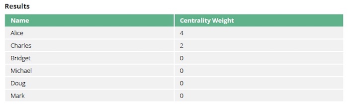
Alice is still the main broker in the network, and Charles is a minor broker, although their centrality score has dropped as the algorithm only considers relationships at a depth of 1. The others don’t have any influence, because all the shortest paths between pairs of people go via Alice or Charles.
Conclusion
As we showed in our look at the Betweenness Centrality algorithm, Betweenness Centrality applies to a wide range of problems in network science and pinpoints bottlenecks or vulnerabilities in communication and transportation networks.Next week we’ll continue our look at Centrality algorithms, with a focus on the Closeness Centrality algorithm.
Find the patterns in your connected data
Learn about the power of graph algorithms in the O’Reilly book,
Graph Algorithms: Practical Examples in Apache Spark and Neo4j by the authors of this article. Click below to get your free ebook copy.
Get the O’Reilly Ebook
Learn about the power of graph algorithms in the O’Reilly book,
Graph Algorithms: Practical Examples in Apache Spark and Neo4j by the authors of this article. Click below to get your free ebook copy.
Get the O’Reilly Ebook


