We continue on from our previously loaded data of NYC bus delays. Although we are fairly sure that our target variable (time_delayed) is not accurate, it is all we have. We can thank the bus drivers of New York that we have anything at all, I suppose, but the inaccuracy of this variable is probably one of the reasons not very many people have touched this data set.
Data preparation
Some data preparation first. We have initially included the variable 'time_diff_report' in the ii main data set. This is the time between the incident and when the incident is called in to operations. The difficult with this number is that it is obviously included in the time estimate given for the breakdown. The time difference is only ever less than the breakdown time for cases which are reported after they are resolved. Obviously, this number can be used as a strong predictor, while also providing no useful predictive information for our real problem: working out how much longer the bus will be delayed. We correct all of this by subtracting this value from the delayed time, so that 'time_delayed' becomes the amount of time from after operations is called that the bus is delayed. We also remove cases which are resolved before they are reported.
#remove zero variance columns
zero_var <- function(dat) {
  out <- lapply(dat, function(x) length(unique(x)))
  keep <- rownames(data.frame(which(out > 1)))
  dat %>%
    select(keep)
}

in_csv <- "../output/intermediate/ii_spread.csv"
ii_spread <- read_csv(in_csv) %>%
  mutate(
    time_delayed = as.numeric(time_delayed - time_diff_report),
    time_diff_report = NULL
  ) %>%
  filter(reported_before_resolved == 1) %>%
  select(-School_Year, -Route_Number, -Schools_Serviced, -Bus_Company_Name, -Occurred_On) %>%
  zero_var

halfFold <- createFolds(ii_spread$time_delayed, k = 5, list=TRUE)
ii_small <- ii_spread[halfFold[[2]],]
ii_test <-ii_spread[halfFold[[3]],]
ii_train <- ii_spread %>%
  anti_join(ii_test, by = "Busbreakdown_ID")

rctrl_manual <- trainControl(method = "none", returnResamp = "all")
rctrl_repcv <- trainControl(method = "repeatedcv", number = 2, repeats = 5, returnResamp = "all")
Cross fold validation testing
Since I am running all of this locally on a laptop which 'benchmarkme' tells me is the slowest system to have been benchmarked in 2018, I build data set 'ii_small' to do cross-fold validation testing, with root mean square error as my target. During my run, I test different numbers of committees and rules. The numbers presented here are what I ended up with. Neighbours always degrade the solution in this case are fixed to zero. We can see the full rule set of the model by calling 'summary', but this results in a lot of spam. A more succinct presentation is available by looking at the 'finalModel' components of the derived model. 'splits' gives a list of the derived rules, where multiple entries per rule indicates an 'AND' condition (both conditions satisfied). 'coefficients' gives the resulting slope and intercept of the application of that rule. Finally, we can get a full listing of how many times a predictor appears in the ruleset and the coefficient set by looking at 'usage': this is somewhat equivalent to a variable importance call.
#---cubist
cubist_grd <- expand.grid(
  committees = 1,
  neighbors = 0
)

set.seed(849)
cubist_cv <- train(time_delayed ~ . -Busbreakdown_ID,
  data = ii_small,
  method = "cubist",
  metric="RMSE",
  na.action = na.pass,
  trControl = rctrl_repcv,
  tuneGrid = cubist_grd,
  control = Cubist::cubistControl(unbiased = T, rules = 20, sample = 0)
)
cubist_cv
## Cubist
##
## 40908 samples
##    25 predictor
##
## No pre-processing
## Resampling: Cross-Validated (2 fold, repeated 5 times)
## Summary of sample sizes: 20454, 20454, 20453, 20455, 20455, 20453, ...
## Resampling results:
##
##   RMSE      Rsquared   MAE
##   13.52728  0.1336734  9.883126
##
## Tuning parameter 'committees' was held constant at a value of 1
##
## Tuning parameter 'neighbors' was held constant at a value of 0
#summary(cubist_cv)
cubist_cv$finalModel$splits %>% glimpse
## Observations: 89
## Variables: 8
## $ committee  <dbl> 1, 1, 1, 1, 1, 1, 1, 1, 1, 1, 1, 1, 1, 1, 1, 1, 1, ...
## $ rule       <dbl> 1, 1, 1, 1, 2, 3, 3, 4, 4, 4, 5, 5, 5, 5, 5, 5, 6, ...
## $ variable   <fct> School_Age, Boro_Bronx, Reason_HeavyTraffic, Number...
## $ dir        <fct> <=, <=, >, <=, >, >, >, >, <=, >, <=, >, <=, <=, <=...
## $ value      <dbl> 0, 0, 0, 6, 0, 0, 0, 3, 0, 0, 0, 0, 0, 0, 0, 0, 0, ...
## $ category   <fct> , , , , , , , , , , , , , , , , , , , , , , , ,
## $ type       <chr> "type2", "type2", "type2", "type2", "type2", "type2...
## $ percentile <dbl> 0.13063459, 0.75171116, 0.29549232, 0.88540139, 0.9...
cubist_cv$finalModel$coefficients %>% glimpse
## Observations: 20
## Variables: 27
## $ `(Intercept)`                   <dbl> 16.8, 14.9, 13.8, 21.0, 14.7, ...
## $ Has_Contractor_Notified_Schools <dbl> NA, NA, 1.4, 8.7, 1.4, 2.2, NA...
## $ Has_Contractor_Notified_Parents <dbl> NA, 7.2, 4.0, -7.9, NA, 1.2, 3...
## $ Have_You_Alerted_OPT            <dbl> NA, 6.1, NA, -2.6, NA, -1.9, 3...
## $ Number_Of_Students_On_The_Bus   <dbl> -0.78, -0.56, -0.17, -0.70, -0...
## $ School_Age                      <dbl> NA, NA, NA, -1.2, NA, -2.3, 5....
## $ Reason_Accident                 <dbl> NA, NA, 10, 2, NA, 6, 10, NA, ...
## $ Reason_DelayedbySchool          <dbl> NA, NA, NA, NA, NA, -5, -5, NA...
## $ Reason_FlatTire                 <dbl> NA, NA, 7, 1, NA, 4, NA, NA, 1...
## $ Reason_HeavyTraffic             <dbl> NA, NA, -2.0, 1.9, NA, -1.2, N...
## $ Reason_LatereturnfromFieldTrip  <dbl> NA, NA, NA, NA, NA, 2.1, 5.6, ...
## $ Reason_MechanicalProblem        <dbl> NA, NA, 6.7, 14.6, NA, 5.0, 6....
## $ Reason_ProblemRun               <dbl> NA, NA, NA, NA, NA, 2, 8, NA, ...
## $ Reason_WeatherConditions        <dbl> NA, NA, 10.3, 3.6, NA, 3.4, NA...
## $ Reason_WontStart                <dbl> NA, NA, NA, NA, NA, 2, NA, NA,...
## $ Boro_Bronx                      <dbl> NA, NA, NA, NA, NA, -2.5, NA, ...
## $ Boro_Brooklyn                   <dbl> NA, 0.4, NA, NA, 3.7, 1.1, 4.8...
## $ Boro_Connecticut                <dbl> NA, NA, NA, NA, NA, NA, NA, NA...
## $ Boro_Manhattan                  <dbl> NA, 0.6, NA, NA, NA, 2.6, 4.3,...
## $ Boro_NassauCounty               <dbl> NA, NA, NA, NA, 8, 3, NA, NA, ...
## $ Boro_NewJersey                  <dbl> NA, NA, NA, NA, NA, 4, 5, NA, ...
## $ Boro_Queens                     <dbl> NA, 0.5, NA, NA, 6.8, 2.2, 3.6...
## $ Boro_RocklandCounty             <dbl> NA, NA, NA, NA, NA, 4, NA, NA,...
## $ Boro_StatenIsland               <dbl> NA, NA, NA, NA, NA, -2.5, NA, ...
## $ Boro_Westchester                <dbl> NA, 1.2, NA, NA, NA, 5.1, 13.6...
## $ committee                       <chr> "1", "1", "1", "1", "1", "1", ...
## $ rule                            <chr> "1", "2", "3", "4", "5", "6", ...
cubist_cv$finalModel$usage %>% head
##   Conditions Model                        Variable
## 1         68    98   Number_Of_Students_On_The_Bus
## 2         66     6                      Boro_Bronx
## 3         65    29             Reason_HeavyTraffic
## 4         52    79 Has_Contractor_Notified_Parents
## 5         46    45                      School_Age
## 6         38    47                  Boro_Manhattan
Validation on test data
We could look through this data set for human-readable rules, but we can see from the high RMSE and low \(R^2\) value that we do not have a very good fit. To look at exactly how rough a model this is, we use our manual fold splits to predict from our 'ii_test' data set:
cubist_man <- train(time_delayed ~ . -Busbreakdown_ID,
  data = ii_train,
  method = "cubist",
  metric="RMSE",
  na.action = na.pass,
  trControl = rctrl_manual,
  tuneGrid = cubist_grd,
  control = Cubist::cubistControl(unbiased = T, rules = 20, sample = 0)
)

ii_withpred <- ii_test %>%
  mutate(
    time_predicted = predict(cubist_man, newdata = ii_test)
  )

ii_withpred %>%
  summarise(
    rms = (mean((time_predicted-time_delayed)^2))^0.5,
    sum_sq = sum((time_predicted-time_delayed)^2),
    tot_sum_sq = sum((time_delayed - mean(time_delayed))^2),
    r_sq = 1- sum_sq / tot_sum_sq
  ) #1,20: 13.5, 0.141
## # A tibble: 1 x 4
##     rms   sum_sq tot_sum_sq  r_sq
##   <dbl>    <dbl>      <dbl> <dbl>
## 1  13.6 7542210.   8829766. 0.146
protec <- ii_withpred %>%
  mutate(Reason_Other = 1L) %>% #dummy flag to get the name in
  select(-contains("Reason")) %>%
  colnames()

pal <- brewer.pal(10, "Paired")

ii_withpred %>%
  mutate(Reason_Other = ifelse(Reason_Accident + Reason_DelayedbySchool + Reason_FlatTire + Reason_HeavyTraffic + Reason_LatereturnfromFieldTrip + Reason_MechanicalProblem + Reason_ProblemRun + Reason_WeatherConditions + Reason_WontStart == 1, 0L, 1L)) %>%
  gather(key = Reason, value = dummy, -one_of(protec)) %>%
  filter(dummy == 1) %>%
  mutate(dummy = NULL) %>%
  filter(row_number() %% 10 == 0) %>%
  ggplot(aes(x = time_predicted, y = time_delayed, fill = Reason, color = Reason)) +
  geom_point(alpha = 0.75, shape = 21) +
  scale_fill_manual(values = pal) +
  geom_abline(intercept = 0, slope = 1, color = "red") +
  coord_cartesian(expand = c(0,0), x = c(0,60)) +
  theme_classic() +
  labs(x="time_predicted [min]",y="time_delayed [min]") +
  theme(text=element_text(family="Arial", size=16)) +
  theme(axis.line = element_line(colour = 'black', size = 1)) +
  theme(axis.ticks = element_line(colour = "black", size = 1)) +
  ggtitle("Simple Cubist: delayed vs predicted")
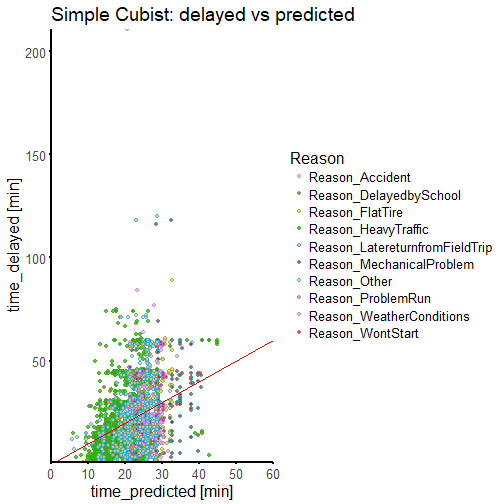
We can see that we haven't done a very good job. We are mis-predicting pretty much everything. But that is fine, since we know that we have more predictors available that we have not yet joined to the data set: company and route level metadata. We also do not know whether a regression approach is really going to be useful with this data, and indeed, later on we will switch over to a two class classification problem, and simply look at whether a delay will be greater or less than a cut off time.