In this post, I will briefly review the basic theory about Ordinary Linear Regression (OLR) using the frequentist approach and from it introduce the Bayesian approach. This will lay the terrain for a later post about Gaussian Processes. The reader may ask himself why “Ordinary Linear Regression” instead of “Ordinary Least Squares.” The answer is that least squares refers to the objective function to be minimized, the sum of the square errors, which is not used the Bayesian approach presented here. I want to thank Jared Smith and Jon Lamontagne for reviewing and improving this post. This post closely follows the presentation in Murphy (2012), which for some reason does not use “^” to denote estimated quantities (if you know why, please leave a comment).
Ordinary Linear Regression
OLR is used to fit a model that is linear in the parameters to a data set  , where
  represents the independent variables and
  the dependent variable, and has the form
where  is a vector of model parameters and
  is the model error variance. The unusual notation for the normal distribution
  should be read as “a normal distribution of with (or given) mean
  and variance .” One frequentist method of estimating the parameters of a linear regression model is the method of maximum likelihood estimation (MLE). MLE provides point estimates
  for each of the regression model parameters by maximizing the likelihood function with respect to and by solving the maximization problem
where the likelihood function  is defined as
where  is the mean of the model error (normally
  ),
),  is the number of points in the data set,
  is an identity matrix, and
  is a vector of values of the independent variables for an individual data point of matrix . OLR assumes independence and the same model error variance among observations, which is expressed by the covariance matrix
  . Digression: in Generalized Linear Regression (GLR), observations may not be independent and may have different variances (heteroscedasticity), so the covariance matrix may have off-diagonal terms and the diagonal terms may not be equal.
If a non-linear function shape is sought, linear regression can be used to fit a model linear in the parameters over a function  of the data — I am not sure why the machine learning community chose
  for this function, but do not confuse it with a normal distribution. This procedure is called basis function expansion and has a likelihood function of the form

where  can have, for example, the form

for fitting a parabola to a one-dimensional over . When minimizing the squared residuals we get to the famous Ordinary Least Squares regression. Linear regression can be further developed, for example, into Ridge Regression to better handle multicollinearity by introducing bias to the parameter estimates, and into Kernel Ridge regression to implicitly add non-linear terms to the model. These formulations are beyond the scope of this post.
What is important to notice is that the standard approaches for linear regression described here, although able to fit linear and non-linear functions, do not provide much insight into the model errors. That is when Bayesian methods come to play.
Bayesian Ordinary Linear Regression
In Bayesian Linear regression (and in any Bayesian approach), the parameters are treated themselves as random variables. This allows for the consideration of model uncertainty, given that now instead of having the best point estimates for we have their full distributions from which to sample models — a sample of corresponds to a model. The distribution of parameters ,  , called the parameter posterior distribution, is calculated by multiplying the likelihood function used in MLE by a prior distribution for the parameters. A prior distribution is assumed from knowledge prior to analyzing new data. In Bayesian Linear Regression, a Gaussian distribution is commonly assumed for the parameters. For example, the prior on can be
  for algebraic simplicity. The parameter posterior distribution assuming a known then has the form
 , given
  is a constant depending only on the data.
We now have an expression from which to derive our parameter posterior for our linear model from which to sample . If the likelihood and the prior are Gaussian, the parameter posterior will also be a Gaussian, given by

where

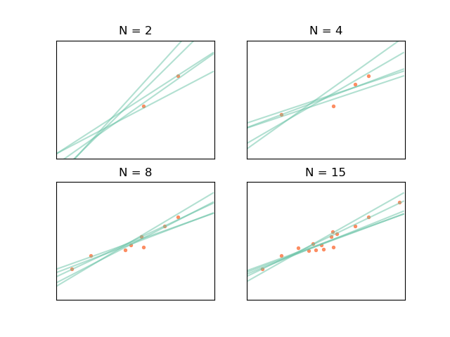
If we calculate the parameter posterior (distribution over parameters ) for a simple linear model  for a data set
  in which and are approximately linearly related given some noise , we can use it to sample values for . This is equivalent to sampling linear models
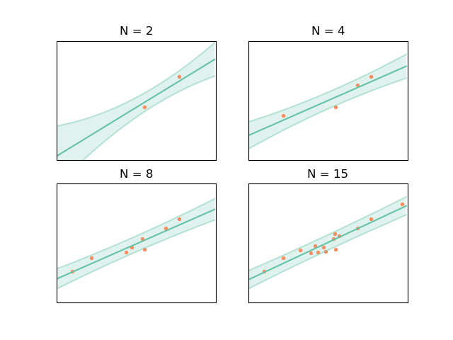
  for data set . As the number of data points increase, the variability of the sampled models should decrease, as in the figure below
This is all interesting but the parameter posterior per se is not of much use. We can, however, use the parameter posterior to find the posterior predictive distribution, which can be used to both get point estimates of  and the associated error. This is done by multiplying the likelihood by the parameter posterior and marginalizing the result over . This is equivalent to performing infinite sampling of blue lines in the example before to form density functions around a point estimate of
  , with
  denoting a new point that is not in . If the likelihood and the parameter posterior are Gaussian, the posterior predictive then takes the form below and will also be Gaussian (in Bayesian parlance, this means that the Gaussian distribution is conjugate to itself)!
where
or, to put it simply,

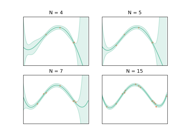
The posterior predictive, meaning final linear model and associated errors (the parameter uncertainty equivalent of frequentist statistics confidence intervals) are shown below
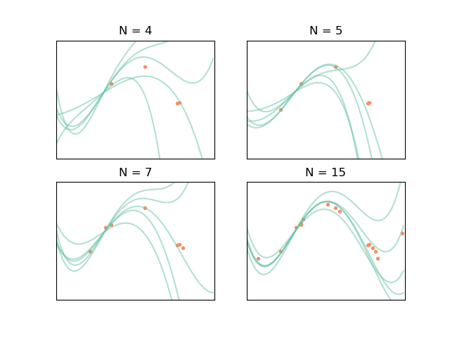
If, instead of having a data set in which and are related approximately according to a 4th order polynomial, we use a function to artificially create more random variables (or features, in machine learning parlance) corresponding to the non-linear terms of the polynomial function. Our function would be ![\phi(x) = [1, x, x^2, x^3, x^4]^T](https://s0.wp.com/latex.php?latex=%5Cphi%28x%29+%3D+%5B1%2C+x%2C+x%5E2%2C+x%5E3%2C+x%5E4%5D%5ET&bg=ffffff&fg=444444&s=0&c=20201002) and the resulting
and the resulting  would therefore have five columns instead of two (
![[1, x]^T](https://s0.wp.com/latex.php?latex=%5B1%2C+x%5D%5ET&bg=ffffff&fg=444444&s=0&c=20201002) ), so now the task is to find
), so now the task is to find ![\boldsymbol{\beta}=[\beta_0, \beta_1, \beta_2, \beta_3, \beta_4]^T](https://s0.wp.com/latex.php?latex=%5Cboldsymbol%7B%5Cbeta%7D%3D%5B%5Cbeta_0%2C+%5Cbeta_1%2C+%5Cbeta_2%2C+%5Cbeta_3%2C+%5Cbeta_4%5D%5ET&bg=ffffff&fg=444444&s=0&c=20201002) . Following the same logic as before for
. Following the same logic as before for  and
and  , where prime denotes the new set random variable
  from function , we get the following plots
This looks great, but there is a problem: what if we do not know the functional form of the model we are supposed to fit (e.g. a simple linear function or a 4th order polynomial)? This is often the case, such as when modeling the reliability of a water reservoir system contingent on stored volumes, inflows and evaporation rates, or when modeling topography based on samples surveyed points (we do not have detailed elevation information about the terrain, e.g. a DEM file). Gaussian Processes (GPs) provide a way of going around this difficulty.
References
Murphy, Kevin P., 2012. Machine Learning: A Probabilistic Perspective. The MIT Press.


Pingback: Introduction to Gaussian Processes – Water Programming: A Collaborative Research Blog