
Given the rise of smart electricity meters and the wide adoption of electricity generation technology like solar panels, there is a wealth of electricity usage data available.
This data represents a multivariate time series of power-related variables that in turn could be used to model and even forecast future electricity consumption.
In this tutorial, you will discover how to develop a test harness for the ‘household power consumption’ dataset and evaluate three naive forecast strategies that provide a baseline for more sophisticated algorithms.
After completing this tutorial, you will know:
- How to load, prepare, and downsample the household power consumption dataset ready for developing models.
- How to develop metrics, dataset split, and walk-forward validation elements for a robust test harness for evaluating forecasting models.
- How to develop and evaluate and compare the performance a suite of naive persistence forecasting methods.
Kick-start your project with my new book Deep Learning for Time Series Forecasting, including step-by-step tutorials and the Python source code files for all examples.
Let’s get started.

How to Develop and Evaluate Naive Forecast Methods for Forecasting Household Electricity Consumption
Photo by Philippe Put, some rights reserved.
Tutorial Overview
This tutorial is divided into four parts; they are:
- Problem Description
- Load and Prepare Dataset
- Model Evaluation
- Naive Forecast Models
Problem Description
The ‘Household Power Consumption‘ dataset is a multivariate time series dataset that describes the electricity consumption for a single household over four years.
The data was collected between December 2006 and November 2010 and observations of power consumption within the household were collected every minute.
It is a multivariate series comprised of seven variables (besides the date and time); they are:
- global_active_power: The total active power consumed by the household (kilowatts).
- global_reactive_power: The total reactive power consumed by the household (kilowatts).
- voltage: Average voltage (volts).
- global_intensity: Average current intensity (amps).
- sub_metering_1: Active energy for kitchen (watt-hours of active energy).
- sub_metering_2: Active energy for laundry (watt-hours of active energy).
- sub_metering_3: Active energy for climate control systems (watt-hours of active energy).
Active and reactive energy refer to the technical details of alternative current.
A fourth sub-metering variable can be created by subtracting the sum of three defined sub-metering variables from the total active energy as follows:
|
1 |
sub_metering_remainder = (global_active_power * 1000 / 60) - (sub_metering_1 + sub_metering_2 + sub_metering_3) |
Load and Prepare Dataset
The dataset can be downloaded from the UCI Machine Learning repository as a single 20 megabyte .zip file:
Download the dataset and unzip it into your current working directory. You will now have the file “household_power_consumption.txt” that is about 127 megabytes in size and contains all of the observations.
We can use the read_csv() function to load the data and combine the first two columns into a single date-time column that we can use as an index.
|
1 2 |
# load all data dataset = read_csv('household_power_consumption.txt', sep=';', header=0, low_memory=False, infer_datetime_format=True, parse_dates={'datetime':[0,1]}, index_col=['datetime']) |
Next, we can mark all missing values indicated with a ‘?‘ character with a NaN value, which is a float.
This will allow us to work with the data as one array of floating point values rather than mixed types (less efficient.)
|
1 2 3 4 |
# mark all missing values dataset.replace('?', nan, inplace=True) # make dataset numeric dataset = dataset.astype('float32') |
We also need to fill in the missing values now that they have been marked.
A very simple approach would be to copy the observation from the same time the day before. We can implement this in a function named fill_missing() that will take the NumPy array of the data and copy values from exactly 24 hours ago.
|
1 2 3 4 5 6 7 |
# fill missing values with a value at the same time one day ago def fill_missing(values): one_day = 60 * 24 for row in range(values.shape[0]): for col in range(values.shape[1]): if isnan(values[row, col]): values[row, col] = values[row - one_day, col] |
We can apply this function directly to the data within the DataFrame.
|
1 2 |
# fill missing fill_missing(dataset.values) |
Now we can create a new column that contains the remainder of the sub-metering, using the calculation from the previous section.
|
1 2 3 |
# add a column for for the remainder of sub metering values = dataset.values dataset['sub_metering_4'] = (values[:,0] * 1000 / 60) - (values[:,4] + values[:,5] + values[:,6]) |
We can now save the cleaned-up version of the dataset to a new file; in this case we will just change the file extension to .csv and save the dataset as ‘household_power_consumption.csv‘.
|
1 2 |
# save updated dataset dataset.to_csv('household_power_consumption.csv') |
Tying all of this together, the complete example of loading, cleaning-up, and saving the dataset is listed below.
|
1 2 3 4 5 6 7 8 9 10 11 12 13 14 15 16 17 18 19 20 21 22 23 24 25 26 27 |
# load and clean-up data from numpy import nan from numpy import isnan from pandas import read_csv from pandas import to_numeric # fill missing values with a value at the same time one day ago def fill_missing(values): one_day = 60 * 24 for row in range(values.shape[0]): for col in range(values.shape[1]): if isnan(values[row, col]): values[row, col] = values[row - one_day, col] # load all data dataset = read_csv('household_power_consumption.txt', sep=';', header=0, low_memory=False, infer_datetime_format=True, parse_dates={'datetime':[0,1]}, index_col=['datetime']) # mark all missing values dataset.replace('?', nan, inplace=True) # make dataset numeric dataset = dataset.astype('float32') # fill missing fill_missing(dataset.values) # add a column for for the remainder of sub metering values = dataset.values dataset['sub_metering_4'] = (values[:,0] * 1000 / 60) - (values[:,4] + values[:,5] + values[:,6]) # save updated dataset dataset.to_csv('household_power_consumption.csv') |
Running the example creates the new file ‘household_power_consumption.csv‘ that we can use as the starting point for our modeling project.
Need help with Deep Learning for Time Series?
Take my free 7-day email crash course now (with sample code).
Click to sign-up and also get a free PDF Ebook version of the course.
Model Evaluation
In this section, we will consider how we can develop and evaluate predictive models for the household power dataset.
This section is divided into four parts; they are:
- Problem Framing
- Evaluation Metric
- Train and Test Sets
- Walk-Forward Validation
Problem Framing
There are many ways to harness and explore the household power consumption dataset.
In this tutorial, we will use the data to explore a very specific question; that is:
Given recent power consumption, what is the expected power consumption for the week ahead?
This requires that a predictive model forecast the total active power for each day over the next seven days.
Technically, this framing of the problem is referred to as a multi-step time series forecasting problem, given the multiple forecast steps. A model that makes use of multiple input variables may be referred to as a multivariate multi-step time series forecasting model.
A model of this type could be helpful within the household in planning expenditures. It could also be helpful on the supply side for planning electricity demand for a specific household.
This framing of the dataset also suggests that it would be useful to downsample the per-minute observations of power consumption to daily totals. This is not required, but makes sense, given that we are interested in total power per day.
We can achieve this easily using the resample() function on the pandas DataFrame. Calling this function with the argument ‘D‘ allows the loaded data indexed by date-time to be grouped by day (see all offset aliases). We can then calculate the sum of all observations for each day and create a new dataset of daily power consumption data for each of the eight variables.
The complete example is listed below.
|
1 2 3 4 5 6 7 8 9 10 11 12 |
# resample minute data to total for each day from pandas import read_csv # load the new file dataset = read_csv('household_power_consumption.csv', header=0, infer_datetime_format=True, parse_dates=['datetime'], index_col=['datetime']) # resample data to daily daily_groups = dataset.resample('D') daily_data = daily_groups.sum() # summarize print(daily_data.shape) print(daily_data.head()) # save daily_data.to_csv('household_power_consumption_days.csv') |
Running the example creates a new daily total power consumption dataset and saves the result into a separate file named ‘household_power_consumption_days.csv‘.
We can use this as the dataset for fitting and evaluating predictive models for the chosen framing of the problem.
Evaluation Metric
A forecast will be comprised of seven values, one for each day of the week ahead.
It is common with multi-step forecasting problems to evaluate each forecasted time step separately. This is helpful for a few reasons:
- To comment on the skill at a specific lead time (e.g. +1 day vs +3 days).
- To contrast models based on their skills at different lead times (e.g. models good at +1 day vs models good at days +5).
The units of the total power are kilowatts and it would be useful to have an error metric that was also in the same units. Both Root Mean Squared Error (RMSE) and Mean Absolute Error (MAE) fit this bill, although RMSE is more commonly used and will be adopted in this tutorial. Unlike MAE, RMSE is more punishing of forecast errors.
The performance metric for this problem will be the RMSE for each lead time from day 1 to day 7.
As a short-cut, it may be useful to summarize the performance of a model using a single score in order to aide in model selection.
One possible score that could be used would be the RMSE across all forecast days.
The function evaluate_forecasts() below will implement this behavior and return the performance of a model based on multiple seven-day forecasts.
|
1 2 3 4 5 6 7 8 9 10 11 12 13 14 15 16 17 18 |
# evaluate one or more weekly forecasts against expected values def evaluate_forecasts(actual, predicted): scores = list() # calculate an RMSE score for each day for i in range(actual.shape[1]): # calculate mse mse = mean_squared_error(actual[:, i], predicted[:, i]) # calculate rmse rmse = sqrt(mse) # store scores.append(rmse) # calculate overall RMSE s = 0 for row in range(actual.shape[0]): for col in range(actual.shape[1]): s += (actual[row, col] - predicted[row, col])**2 score = sqrt(s / (actual.shape[0] * actual.shape[1])) return score, scores |
Running the function will first return the overall RMSE regardless of day, then an array of RMSE scores for each day.
Train and Test Sets
We will use the first three years of data for training predictive models and the final year for evaluating models.
The data in a given dataset will be divided into standard weeks. These are weeks that begin on a Sunday and end on a Saturday.
This is a realistic and useful way for using the chosen framing of the model, where the power consumption for the week ahead can be predicted. It is also helpful with modeling, where models can be used to predict a specific day (e.g. Wednesday) or the entire sequence.
We will split the data into standard weeks, working backwards from the test dataset.
The final year of the data is in 2010 and the first Sunday for 2010 was January 3rd. The data ends in mid November 2010 and the closest final Saturday in the data is November 20th. This gives 46 weeks of test data.
The first and last rows of daily data for the test dataset are provided below for confirmation.
|
1 2 3 |
2010-01-03,2083.4539999999984,191.61000000000055,350992.12000000034,8703.600000000033,3842.0,4920.0,10074.0,15888.233355799992 ... 2010-11-20,2197.006000000004,153.76800000000028,346475.9999999998,9320.20000000002,4367.0,2947.0,11433.0,17869.76663959999 |
The daily data starts in late 2006.
The first Sunday in the dataset is December 17th, which is the second row of data.
Organizing the data into standard weeks gives 159 full standard weeks for training a predictive model.
|
1 2 3 |
2006-12-17,3390.46,226.0059999999994,345725.32000000024,14398.59999999998,2033.0,4187.0,13341.0,36946.66673200004 ... 2010-01-02,1309.2679999999998,199.54600000000016,352332.8399999997,5489.7999999999865,801.0,298.0,6425.0,14297.133406600002 |
The function split_dataset() below splits the daily data into train and test sets and organizes each into standard weeks.
Specific row offsets are used to split the data using knowledge of the dataset. The split datasets are then organized into weekly data using the NumPy split() function.
|
1 2 3 4 5 6 7 8 |
# split a univariate dataset into train/test sets def split_dataset(data): # split into standard weeks train, test = data[1:-328], data[-328:-6] # restructure into windows of weekly data train = array(split(train, len(train)/7)) test = array(split(test, len(test)/7)) return train, test |
We can test this function out by loading the daily dataset and printing the first and last rows of data from both the train and test sets to confirm they match the expectations above.
The complete code example is listed below.
|
1 2 3 4 5 6 7 8 9 10 11 12 13 14 15 16 17 18 19 20 21 22 23 |
# split into standard weeks from numpy import split from numpy import array from pandas import read_csv # split a univariate dataset into train/test sets def split_dataset(data): # split into standard weeks train, test = data[1:-328], data[-328:-6] # restructure into windows of weekly data train = array(split(train, len(train)/7)) test = array(split(test, len(test)/7)) return train, test # load the new file dataset = read_csv('household_power_consumption_days.csv', header=0, infer_datetime_format=True, parse_dates=['datetime'], index_col=['datetime']) train, test = split_dataset(dataset.values) # validate train data print(train.shape) print(train[0, 0, 0], train[-1, -1, 0]) # validate test print(test.shape) print(test[0, 0, 0], test[-1, -1, 0]) |
Running the example shows that indeed the train dataset has 159 weeks of data, whereas the test dataset has 46 weeks.
We can see that the total active power for the train and test dataset for the first and last rows match the data for the specific dates that we defined as the bounds on the standard weeks for each set.
|
1 2 3 4 |
(159, 7, 8) 3390.46 1309.2679999999998 (46, 7, 8) 2083.4539999999984 2197.006000000004 |
Walk-Forward Validation
Models will be evaluated using a scheme called walk-forward validation.
This is where a model is required to make a one week prediction, then the actual data for that week is made available to the model so that it can be used as the basis for making a prediction on the subsequent week. This is both realistic for how the model may be used in practice and beneficial to the models allowing them to make use of the best available data.
We can demonstrate this below with separation of input data and output/predicted data.
|
1 2 3 4 5 |
Input, Predict [Week1] Week2 [Week1 + Week2] Week3 [Week1 + Week2 + Week3] Week4 ... |
The walk-forward validation approach to evaluating predictive models on this dataset is implement below, named evaluate_model().
The name of a function is provided for the model as the argument “model_func“. This function is responsible for defining the model, fitting the model on the training data, and making a one-week forecast.
The forecasts made by the model are then evaluated against the test dataset using the previously defined evaluate_forecasts() function.
|
1 2 3 4 5 6 7 8 9 10 11 12 13 14 15 16 17 |
# evaluate a single model def evaluate_model(model_func, train, test): # history is a list of weekly data history = [x for x in train] # walk-forward validation over each week predictions = list() for i in range(len(test)): # predict the week yhat_sequence = model_func(history) # store the predictions predictions.append(yhat_sequence) # get real observation and add to history for predicting the next week history.append(test[i, :]) predictions = array(predictions) # evaluate predictions days for each week score, scores = evaluate_forecasts(test[:, :, 0], predictions) return score, scores |
Once we have the evaluation for a model, we can summarize the performance.
The function below named summarize_scores() will display the performance of a model as a single line for easy comparison with other models.
|
1 2 3 4 |
# summarize scores def summarize_scores(name, score, scores): s_scores = ', '.join(['%.1f' % s for s in scores]) print('%s: [%.3f] %s' % (name, score, s_scores)) |
We now have all of the elements to begin evaluating predictive models on the dataset.
Naive Forecast Models
It is important to test naive forecast models on any new prediction problem.
The results from naive models provide a quantitative idea of how difficult the forecast problem is and provide a baseline performance by which more sophisticated forecast methods can be evaluated.
In this section, we will develop and compare three naive forecast methods for the household power prediction problem; they are:
- Daily Persistence Forecast.
- Weekly Persistent Forecast.
- Weekly One-Year-Ago Persistent Forecast.
Daily Persistence Forecast
The first naive forecast that we will develop is a daily persistence model.
This model takes the active power from the last day prior to the forecast period (e.g. Saturday) and uses it as the value of the power for each day in the forecast period (Sunday to Saturday).
The daily_persistence() function below implements the daily persistence forecast strategy.
|
1 2 3 4 5 6 7 8 9 |
# daily persistence model def daily_persistence(history): # get the data for the prior week last_week = history[-1] # get the total active power for the last day value = last_week[-1, 0] # prepare 7 day forecast forecast = [value for _ in range(7)] return forecast |
Weekly Persistent Forecast
Another good naive forecast when forecasting a standard week is to use the entire prior week as the forecast for the week ahead.
It is based on the idea that next week will be very similar to this week.
The weekly_persistence() function below implements the weekly persistence forecast strategy.
|
1 2 3 4 5 |
# weekly persistence model def weekly_persistence(history): # get the data for the prior week last_week = history[-1] return last_week[:, 0] |
Weekly One-Year-Ago Persistent Forecast
Similar to the idea of using last week to forecast next week is the idea of using the same week last year to predict next week.
That is, use the week of observations from 52 weeks ago as the forecast, based on the idea that next week will be similar to the same week one year ago.
The week_one_year_ago_persistence() function below implements the week one year ago forecast strategy.
|
1 2 3 4 5 |
# week one year ago persistence model def week_one_year_ago_persistence(history): # get the data for the prior week last_week = history[-52] return last_week[:, 0] |
Naive Model Comparison
We can compare each of the forecast strategies using the test harness developed in the previous section.
First, the dataset can be loaded and split into train and test sets.
|
1 2 3 4 |
# load the new file dataset = read_csv('household_power_consumption_days.csv', header=0, infer_datetime_format=True, parse_dates=['datetime'], index_col=['datetime']) # split into train and test train, test = split_dataset(dataset.values) |
Each of the strategies can be stored in a dictionary against a unique name. This name can be used in printing and in creating a plot of the scores.
|
1 2 3 4 5 |
# define the names and functions for the models we wish to evaluate models = dict() models['daily'] = daily_persistence models['weekly'] = weekly_persistence models['week-oya'] = week_one_year_ago_persistence |
We can then enumerate each of the strategies, evaluating it using walk-forward validation, printing the scores, and adding the scores to a line plot for visual comparison.
|
1 2 3 4 5 6 7 8 9 |
# evaluate each model days = ['sun', 'mon', 'tue', 'wed', 'thr', 'fri', 'sat'] for name, func in models.items(): # evaluate and get scores score, scores = evaluate_model(func, train, test) # summarize scores summarize_scores('daily persistence', score, scores) # plot scores pyplot.plot(days, scores, marker='o', label=name) |
Tying all of this together, the complete example evaluating the three naive forecast strategies is listed below.
|
1 2 3 4 5 6 7 8 9 10 11 12 13 14 15 16 17 18 19 20 21 22 23 24 25 26 27 28 29 30 31 32 33 34 35 36 37 38 39 40 41 42 43 44 45 46 47 48 49 50 51 52 53 54 55 56 57 58 59 60 61 62 63 64 65 66 67 68 69 70 71 72 73 74 75 76 77 78 79 80 81 82 83 84 85 86 87 88 89 90 91 92 93 94 95 96 97 98 99 100 101 102 |
# naive forecast strategies from math import sqrt from numpy import split from numpy import array from pandas import read_csv from sklearn.metrics import mean_squared_error from matplotlib import pyplot # split a univariate dataset into train/test sets def split_dataset(data): # split into standard weeks train, test = data[1:-328], data[-328:-6] # restructure into windows of weekly data train = array(split(train, len(train)/7)) test = array(split(test, len(test)/7)) return train, test # evaluate one or more weekly forecasts against expected values def evaluate_forecasts(actual, predicted): scores = list() # calculate an RMSE score for each day for i in range(actual.shape[1]): # calculate mse mse = mean_squared_error(actual[:, i], predicted[:, i]) # calculate rmse rmse = sqrt(mse) # store scores.append(rmse) # calculate overall RMSE s = 0 for row in range(actual.shape[0]): for col in range(actual.shape[1]): s += (actual[row, col] - predicted[row, col])**2 score = sqrt(s / (actual.shape[0] * actual.shape[1])) return score, scores # summarize scores def summarize_scores(name, score, scores): s_scores = ', '.join(['%.1f' % s for s in scores]) print('%s: [%.3f] %s' % (name, score, s_scores)) # evaluate a single model def evaluate_model(model_func, train, test): # history is a list of weekly data history = [x for x in train] # walk-forward validation over each week predictions = list() for i in range(len(test)): # predict the week yhat_sequence = model_func(history) # store the predictions predictions.append(yhat_sequence) # get real observation and add to history for predicting the next week history.append(test[i, :]) predictions = array(predictions) # evaluate predictions days for each week score, scores = evaluate_forecasts(test[:, :, 0], predictions) return score, scores # daily persistence model def daily_persistence(history): # get the data for the prior week last_week = history[-1] # get the total active power for the last day value = last_week[-1, 0] # prepare 7 day forecast forecast = [value for _ in range(7)] return forecast # weekly persistence model def weekly_persistence(history): # get the data for the prior week last_week = history[-1] return last_week[:, 0] # week one year ago persistence model def week_one_year_ago_persistence(history): # get the data for the prior week last_week = history[-52] return last_week[:, 0] # load the new file dataset = read_csv('household_power_consumption_days.csv', header=0, infer_datetime_format=True, parse_dates=['datetime'], index_col=['datetime']) # split into train and test train, test = split_dataset(dataset.values) # define the names and functions for the models we wish to evaluate models = dict() models['daily'] = daily_persistence models['weekly'] = weekly_persistence models['week-oya'] = week_one_year_ago_persistence # evaluate each model days = ['sun', 'mon', 'tue', 'wed', 'thr', 'fri', 'sat'] for name, func in models.items(): # evaluate and get scores score, scores = evaluate_model(func, train, test) # summarize scores summarize_scores(name, score, scores) # plot scores pyplot.plot(days, scores, marker='o', label=name) # show plot pyplot.legend() pyplot.show() |
Running the example first prints the total and daily scores for each model.
We can see that the weekly strategy performs better than the daily strategy and that the week one year ago (week-oya) performs slightly better again.
Note: Your results may vary given the stochastic nature of the algorithm or evaluation procedure, or differences in numerical precision. Consider running the example a few times and compare the average outcome.
We can see this in both the overall RMSE scores for each model and in the daily scores for each forecast day. One exception is the forecast error for the first day (Sunday) where it appears that the daily persistence model performs better than the two weekly strategies.
We can use the week-oya strategy with an overall RMSE of 465.294 kilowatts as the baseline in performance for more sophisticated models to be considered skillful on this specific framing of the problem.
|
1 2 3 |
daily: [511.886] 452.9, 596.4, 532.1, 490.5, 534.3, 481.5, 482.0 weekly: [469.389] 567.6, 500.3, 411.2, 466.1, 471.9, 358.3, 482.0 week-oya: [465.294] 550.0, 446.7, 398.6, 487.0, 459.3, 313.5, 555.1 |
A line plot of the daily forecast error is also created.
We can see the same observed pattern of the weekly strategies performing better than the daily strategy in general, except in the case of the first day.
It is surprising (to me) that the week one-year-ago performs better than using the prior week. I would have expected that the power consumption from last week to be more relevant.
Reviewing all strategies on the same plot suggests possible combinations of the strategies that may result in even better performance.
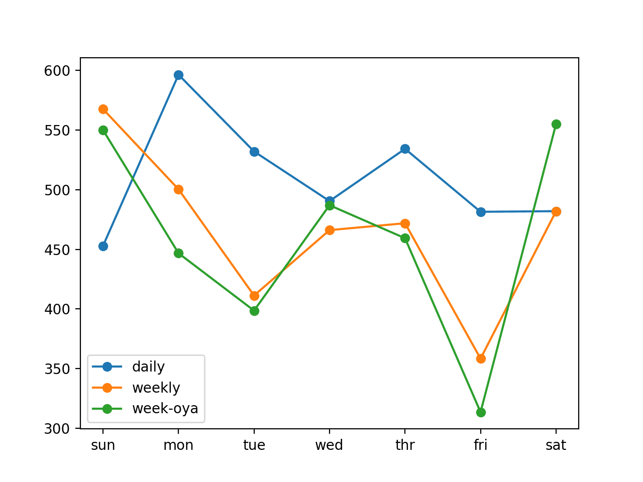
Line Plot Comparing Naive Forecast Strategies for Household Power Forecasting
Extensions
This section lists some ideas for extending the tutorial that you may wish to explore.
- Additional Naive Strategy. Propose, develop, and evaluate one more naive strategy for forecasting the next week of power consumption.
- Naive Ensemble Strategy. Develop an ensemble strategy that combines the predictions from the three proposed naive forecast methods.
- Optimized Direct Persistence Models. Test and find the optimal relative prior day (e.g. -1 or -7) to use for each forecast day in a direct persistence model.
If you explore any of these extensions, I’d love to know.
Further Reading
This section provides more resources on the topic if you are looking to go deeper.
API
- pandas.read_csv API
- pandas.DataFrame.resample API
- Resample Offset Aliases
- sklearn.metrics.mean_squared_error API
- numpy.split API
Articles
- Individual household electric power consumption Data Set, UCI Machine Learning Repository.
- AC power, Wikipedia.
Summary
In this tutorial, you discovered how to develop a test harness for the household power consumption dataset and evaluate three naive forecast strategies that provide a baseline for more sophisticated algorithms.
Specifically, you learned:
- How to load, prepare, and downsample the household power consumption dataset ready for modeling.
- How to develop metrics, dataset split, and walk-forward validation elements for a robust test harness for evaluating forecasting models.
- How to develop and evaluate and compare the performance a suite of naive persistence forecasting methods.
Do you have any questions?
Ask your questions in the comments below and I will do my best to answer.
Develop Deep Learning models for Time Series Today!

Develop Your Own Forecasting models in Minutes
...with just a few lines of python code
Discover how in my new Ebook:
Deep Learning for Time Series Forecasting
It provides self-study tutorials on topics like:
CNNs, LSTMs,
Multivariate Forecasting, Multi-Step Forecasting and much more...
Finally Bring Deep Learning to your Time Series Forecasting Projects
Skip the Academics. Just Results.


hello Jason,
your article is best for us to learn ML AND DL.
do you have any article about reinforcement learning ,such as Sarsa、Q learning、Monte-carlo learning、Deep-Q-Network and so on?
thanks a lot.
Not at this stage, I don’t see how they can be useful on anything other than toy problems (e.g. I don’t see how developers can use the methods “at work”.)
Hi Jason!
I am currently working on a NMT project for translation of my native language to English and vice versa. As told my project mentor I generated 20 epochs with the help of the readme file that comes by default with openNMT package. Now I am asked to generate 80 more epochs. He told that it can be achieved by start_index and end_index. I searched a lot how to do that and finally found this
https://machinelearningmastery.com/text-generation-lstm-recurrent-neural-networks-python-keras/
Please direct me how to do this.!
Thank you
Sorry, I don’t have material on openNMT, I cannot give you good off the cuff advice.
Okay then!
Thanks for your response
thanks for your reply.
have a good day.
No problem.
Great article (and series). Thanks. Is there a version of the code in R?
Thanks.
No, sorry my focus is on Python at the moment given the much greater demand.
transform dataset to household_power_consumption_hour
I use your code.
six hours as one ”benchmark” just like seven days as one week.
Do I understand this correctly?
TANKS
Sorry, I don’t have the capacity to debug your changes.
Hello! Now I want to make a model of the power amplifier. The input and output of the power amplifier are complex Numbers composed of the real part and the imaginary part. Now I have the data of the input and output. What to do with this data, thank you so much
Perhaps try a range of representations and models and see what works best for your specific dataset, this might help:
https://machinelearningmastery.com/faq/single-faq/what-algorithm-config-should-i-use
Can You please mention the detailed conclusion of naive bayes algorithm applied.
We did not use naive bayes in this tutorial.
Overall RMSE could be computed with the formula :
”’python
score = np.sqrt(np.mean((actual-predicted)**2))
”’
For clarity, the dataset should keep only the values that will be predicted (and drop all other columns) and manipulate only numpy arrays (instead of lists)
A nice additional plot would be to the forceasts and real baseline for some period.
Best regards
Thanks.
Excellent contribution, a question if my variable of interest for the prediction was the voltage as an adjustment so that in the prediction it takes this value as output.
Thank you for your cooperation
Sorry, I don’t follow your question, perhaps you can restate it?
How can I change the prediction variable in the code?
in this case select another variable in the dataset (voltage)
Perhaps focus on the “Load and Prepare Dataset” section.
It should be quite straightforward, if not, perhaps start with some simpler tutorials to get familiar with python programming.
Hi Jason,
Thanks for this nice tutorial,
There is something that I couldn’t understand with the way of reshaping the dataset. Actually I have this problem with most of your tutorials. I believe there is a point that I misunderstood.
So The shape of the data after split is as following- train : (159, 7, 8) and test: (46, 7, 8)
so the predictions shape will be (46, 7, 1)? correct?
If so, this means there are more points predicted than needed? aren’t they?
I got something strange when I try to plot the results. I am not sure why!!
here is how it looks like
I https://www.dropbox.com/s/8jblxjhxmtfjcip/Screen%20Shot%202020-06-03%20at%206.23.29%20pm.png?dl=0
your feedback is highly valuable for me.
One more question, is there any discounts if I want to buy a single book from yours?
Regards,
The input shape for LSTMs can be confusing, this will help:
https://machinelearningmastery.com/faq/single-faq/what-is-the-difference-between-samples-timesteps-and-features-for-lstm-input