Introduction
Tribbles originate from the planet Iota Geminorum IV and, according to Dr. McCoy, are born pregnant. No further details are given but we can follow Gurtin and MacCamy (1974) and perhaps recover some of what happens on the Enterprise.
Of course, age-dependent population models are of more than fictional use and can be applied, for example, to modelling the progression of Malaria in infected hosts. We roughly follow some of J. J. Thibodeaux and Schlittenhardt (2011) who themselves reference Belair, Mackey, and Mahaffy (1995).
Of interest to Haskellers are:
-
The use of the hmatrix package which now contains functions to solve tridiagonal systems used in this post. You will need to use HEAD until a new hackage / stackage release is made. My future plan is to use CUDA via accelerate and compare.
-
The use of dimensions in a medium-sized example. It would have been nice to have tried the units package but it seemed harder work to use and, as ever, “Time’s wingèd chariot” was the enemy.
The source for this post can be downloaded from github.
Age-Dependent Populations
McKendrick / von Foerster
McKendrick and von Foerster independently derived a model of age-dependent population growth.
Let 


where 


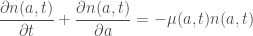
which in the limit becomes

We can further assume that the rate of entry to a cohort is proportional to the density of individuals times a velocity of aging 

Occasionally there is some reason to assume that aging one year is different to experiencing one year but we further assume 
We thus obtain
Gurtin / MacCamy
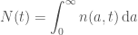
To solve any PDE we need boundary and initial conditions. The number of births at time
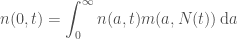
where 
and we further assume that the initial condition

for some given 
Gurtin and MacCamy (1974) focus on the situation where

and we can also assume that the birth rate of Tribbles decreases exponentially with age and further that Tribbles can live forever. Gurtin and MacCamy (1974) then transform the PDE to obtain a pair of linked ODEs which can then be solved numerically.
Of course, we know what happens in the Enterprise and rather than continue with this example, let us turn our attention to the more serious subject of Malaria.
Malaria
I realise now that I went a bit overboard with references. Hopefully they don’t interrupt the flow too much.
The World Health Organisation (WHO) estimated that in 2015 there were 214 million new cases of malaria resulting in 438,000 deaths (source: Wikipedia).
The lifecycle of the plasmodium parasite that causes malaria is extremely ingenious. J. J. Thibodeaux and Schlittenhardt (2011) model the human segment of the plasmodium lifecycle and further propose a way of determing an optimal treatment for an infected individual. Hall et al. (2013) also model the effect of an anti-malarial. Let us content ourselves with reproducing part of the paper by J. J. Thibodeaux and Schlittenhardt (2011).
At one part of its sojourn in humans, plasmodium infects erythrocytes aka red blood cells. These latter contain haemoglobin (aka hemoglobin). The process by which red blood cells are produced, Erythropoiesis, is modulated in a feedback loop by erythropoietin. The plasmodium parasite severely disrupts this process. Presumably the resulting loss of haemoglobin is one reason that an infected individual feels ill.
As can be seen in the overview by Torbett and Friedman (2009), the full feedback loop is complex. So as not to lose ourselves in the details and following J. J. Thibodeaux and Schlittenhardt (2011) and Belair, Mackey, and Mahaffy (1995), we consider a model with two compartments.
-
Precursors: prototype erythrocytes developing in the bone marrow with
being the density of such cells of age
at time
-
Erythrocytes: mature red blood cells circulating in the blood with
being the density of such cells of age
at time

where 


As boundary conditions, we have that the number of precursors maturing must equal the production of number of erythrocytes

and the production of the of the number of precursors depends on the level of erythropoietin

where 
As initial conditions, we have

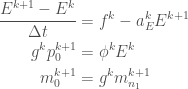
We can further model the erythropoietin dynamics as
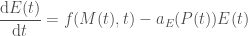
where 


As initial condition we have

A Finite Difference Attempt
Let us try solving the above model using a finite difference scheme observing that we currently have no basis for whether it has a solution and whether the finite difference scheme approximates such a solution! We follow J. J. Thibodeaux and Schlittenhardt (2011) who give a proof of convergence presumably with some conditions; any failure of the scheme is entirely mine.
Divide up the age and time ranges, ![[0, \mu_F]](https://s0.wp.com/latex.php?latex=%5B0%2C+%5Cmu_F%5D&bg=ffffff&fg=444444&s=0&c=20201002)
![[0, \nu_F]](https://s0.wp.com/latex.php?latex=%5B0%2C+%5Cnu_F%5D&bg=ffffff&fg=444444&s=0&c=20201002)
![[0, T]](https://s0.wp.com/latex.php?latex=%5B0%2C+T%5D&bg=ffffff&fg=444444&s=0&c=20201002)
![[\mu_i, \mu_{i+1}]](https://s0.wp.com/latex.php?latex=%5B%5Cmu_i%2C+%5Cmu_%7Bi%2B1%7D%5D&bg=ffffff&fg=444444&s=0&c=20201002)
![[\nu_j, \nu_{j+1}]](https://s0.wp.com/latex.php?latex=%5B%5Cnu_j%2C+%5Cnu_%7Bj%2B1%7D%5D&bg=ffffff&fg=444444&s=0&c=20201002)
![[t_k, t_{k+1}]](https://s0.wp.com/latex.php?latex=%5Bt_k%2C+t_%7Bk%2B1%7D%5D&bg=ffffff&fg=444444&s=0&c=20201002)

where 


Denoting 

and
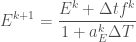
Re-arranging we get

Writing
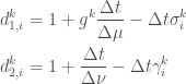
We can express the above in matrix form


Finally we can write
A Haskell Implementation
> {-# OPTIONS_GHC -Wall #-}
> {-# LANGUAGE TypeFamilies #-}
> {-# LANGUAGE NoImplicitPrelude #-}
> {-# LANGUAGE FlexibleContexts #-}
> {-# LANGUAGE DataKinds #-}
> {-# LANGUAGE TypeOperators #-}
> module Tribbles where
> import qualified Prelude as P
> import Numeric.Units.Dimensional.Prelude hiding (Unit)
> import Numeric.Units.Dimensional
> import Numeric.LinearAlgebra
> import Numeric.Integration.TanhSinh
> import Control.Monad.Writer
> import Control.Monad.Loops
Substances like erythropoietin (EPO) are measured in International Units and these cannot be converted to Moles (see Jelkmann (2009) for much more detail) so we have to pretend it really is measured in Moles as there seems to be no easy way to define what the dimensional package calls a base dimension. A typical amount for a person is 15 milli-IU / mill-litre but can reach much higher levels after loss of blood.
> muPerMl :: (Fractional a, Num a) => Unit 'NonMetric DConcentration a
> muPerMl = (milli mole) / (milli litre)
> bigE'0 :: Concentration Double
> bigE'0 = 15.0 *~ muPerMl
Let’s set up our grid. We take these from Ackleh et al. (2006) but note that J. J. Thibodeaux and Schlittenhardt (2011) seem to have 
> deltaT, deltaMu, deltaNu :: Time Double
> deltaT = 0.05 *~ day
> deltaMu = 0.01 *~ day
> deltaNu = 0.05 *~ day
> bigT :: Time Double
> bigT = 100.0 *~ day
> muF, nuF :: Time Double
> muF = 5.9 *~ day
> nuF = 120.0 *~ day
> bigK :: Int
> bigK = floor (bigT / deltaT /~ one)
> n1 :: Int
> n1 = floor (muF / deltaMu /~ one)
> n2 :: Int
> n2 = floor (nuF / deltaNu /~ one)
> ts :: [Time Double]
> ts = take bigK $ 0.0 *~ day : (map (+ deltaT) ts)
The birth rate for precursors
> betaThibodeaux :: Time Double ->
>                   Frequency Double
> betaThibodeaux mu
>   | mu < (0 *~ day) = error "betaThibodeaux: negative age"
>   | mu < (3 *~ day) = (2.773 *~ (one / day))
>   | otherwise       = (0.0 *~ (one /day))
> alphaThibodeaux :: Concentration Double ->
>                    Frequency Double
> alphaThibodeaux e = (0.5 *~ (muPerMl / day)) / ((1 *~ muPerMl) + e)
> sigmaThibodeaux :: Time Double ->
>                    Time Double ->
>                    Concentration Double ->
>                    Frequency Double
> sigmaThibodeaux mu _t e = gThibodeaux e * (betaThibodeaux mu - alphaThibodeaux e)
and an alternative birth rate
> betaAckleh :: Time Double -> Frequency Double
> betaAckleh mu
>   | mu < (0 *~ day) = error "betaAckleh: negative age"
>   | mu < (3 *~ day) = 2.773 *~ (one / day)
>   | otherwise       = 0.000 *~ (one / day)
> sigmaAckleh :: Time Double ->
>                Time Double ->
>                Concentration Double ->
>                Frequency Double
> sigmaAckleh mu _t e = betaAckleh mu * gAckleh e
J. J. Thibodeaux and Schlittenhardt (2011) give the maturation rate of precursors 
> gThibodeaux :: Concentration Double  -> Dimensionless Double
> gThibodeaux e = d / n
>   where
>     n = ((3.02 *~ one) * e + (0.31 *~ muPerMl))
>     d = (30.61 *~ muPerMl) + e
and Ackleh et al. (2006) give this as
> gAckleh :: Concentration Double -> Dimensionless Double
> gAckleh _e = 1.0 *~ one
As in J. J. Thibodeaux and Schlittenhardt (2011) we give quantities in terms of cells per kilogram of body weight. Note that these really are moles on this occasion.
> type CellDensity = Quantity (DAmountOfSubstance / DTime / DMass)
Let’s set the initial conditions.
> p'0 :: Time Double -> CellDensity Double
> p'0 mu' = (1e11 *~ one) * pAux mu'
>   where
>     pAux mu
>       | mu < (0 *~ day) = error "p'0: negative age"
>       | mu < (3 *~ day) = 8.55e-6 *~ (mole / day / kilo gram) *
>                           exp ((2.7519 *~ (one / day)) * mu)
>       | otherwise       = 8.55e-6 *~ (mole / day / kilo gram) *
>                           exp (8.319 *~ one - (0.0211 *~ (one / day)) * mu)
> m_0 :: Time Double -> CellDensity Double
> m_0 nu' = (1e11 *~ one) * mAux nu'
>   where
>     mAux nu
>       | nu < (0 *~ day) = error "m_0: age less than zero"
>       | otherwise       = 0.039827  *~ (mole / day / kilo gram) *
>                           exp (((-0.0083) *~ (one / day)) * nu)
And check that these give plausible results.
> m_0Untyped :: Double -> Double
> m_0Untyped nu = m_0 (nu *~ day) /~ (mole / day / kilo gram)
> p'0Untyped :: Double -> Double
> p'0Untyped mu = p'0 (mu *~ day) /~ (mole / day / kilo gram)
ghci> import Numeric.Integration.TanhSinh
ghci> result $ relative 1e-6 $ parTrap m_0Untyped 0.001 (nuF /~ day)
  3.0260736659043414e11

ghci> result $ relative 1e-6 $ parTrap p'0Untyped 0.001 (muF /~ day)
  1.0453999900927126e10
We can now create the components for the first matrix equation.
> g'0 :: Dimensionless Double
> g'0 = gThibodeaux bigE'0
> d_1'0 :: Int -> Dimensionless Double
> d_1'0 i = (1 *~ one) + (g'0 * deltaT / deltaMu)
>           - deltaT * sigmaThibodeaux ((fromIntegral i *~ one) * deltaMu) undefined bigE'0
> lowers :: [Dimensionless Double]
> lowers = replicate n1 (negate $ g'0 * deltaT / deltaMu)
> diags :: [Dimensionless Double]
> diags = g'0 : map d_1'0 [1..n1]
> uppers :: [Dimensionless Double]
> uppers = replicate n1 (0.0 *~ one)
J. J. Thibodeaux and Schlittenhardt (2011) does not give a definition for 


> s_0 :: Time Double ->
>        Quantity (DAmountOfSubstance / DTime / DMass / DConcentration) Double
> s_0 = const ((1e11 *~ one) * (4.45e-7 *~ (mole / day / kilo gram / muPerMl)))
> b'0 :: [CellDensity Double]
> b'0 = (s_0 (0.0 *~ day) * bigE'0) : (take n1 $ map p'0 (iterate (+ deltaMu) deltaMu))
With these components in place we can now solve the implicit scheme and get the age distribution of precursors after one time step.
> p'1 :: Matrix Double
> p'1 = triDiagSolve (fromList (map (/~ one) lowers))
>                    (fromList (map (/~ one) diags))
>                    (fromList (map (/~ one) uppers))
>                    (((n1 P.+1 )><1) (map (/~ (mole / second / kilo gram)) b'0))
In order to create the components for the second matrix equation, we need the death rates of mature erythrocytes
> gammaThibodeaux :: Time Double ->
>                    Time Double ->
>                    Quantity (DAmountOfSubstance / DMass) Double ->
>                    Frequency Double
> gammaThibodeaux _nu _t _bigM = 0.0083 *~ (one / day)
We note an alternative for the death rate
> gammaAckleh :: Time Double ->
>                Time Double ->
>                Quantity (DAmountOfSubstance / DMass) Double ->
>                Frequency Double
> gammaAckleh _nu _t bigM = (0.01 *~ (kilo gram / mole / day)) * bigM + 0.0001 *~ (one / day)
For the intial mature erythrocyte population we can either use the integral of the initial distribution
> bigM'0 :: Quantity (DAmountOfSubstance / DMass) Double
> bigM'0 = r *~ (mole / kilo gram)
>  where
>    r = result $ relative 1e-6 $ parTrap m_0Untyped 0.001 (nuF /~ day)
ghci> bigM'0
  3.0260736659043414e11 kg^-1 mol
or we can use the sum of the values used in the finite difference approximation
> bigM'0' :: Quantity (DAmountOfSubstance / DMass) Double
> bigM'0' = (* deltaNu) $ sum $ map m_0 $ take n2 $ iterate (+ deltaNu) (0.0 *~ day)
ghci> bigM'0'
  3.026741454719976e11 kg^-1 mol
Finally we can create the components
> d_2'0 :: Int -> Dimensionless Double
> d_2'0 i = (1 *~ one) + (g'0 * deltaT / deltaNu)
>           + deltaT * gammaThibodeaux ((fromIntegral i *~ one) * deltaNu) undefined bigM'0
> lowers2 :: [Dimensionless Double]
> lowers2 = replicate n2 (negate $ deltaT / deltaNu)
> diags2 :: [Dimensionless Double]
> diags2 = (1.0 *~ one) : map d_2'0 [1..n2]
> uppers2 :: [Dimensionless Double]
> uppers2 = replicate n2 (0.0 *~ one)
> b_2'0 :: [CellDensity Double]
> b_2'0 = (g'0 * ((p'1 `atIndex` (n1,0)) *~ (mole / second / kilo gram))) :
>         (take n2 $ map m_0 (iterate (+ deltaNu) deltaNu))
and then solve the implicit scheme to get the distribution of mature erythrocytes one time step ahead
> m'1 :: Matrix Double
> m'1 = triDiagSolve (fromList (map (/~ one) lowers2))
>                    (fromList (map (/~ one) diags2))
>                    (fromList (map (/~ one) uppers2))
>                    (((n2 P.+ 1)><1) (map (/~ (mole / second / kilo gram)) b_2'0))
We need to complete the homeostatic loop by implmenting the feedback from the kidneys to the bone marrow. Ackleh and Thibodeaux (2013) and Ackleh et al. (2006) give
> fAckleh :: Time Double ->
>            Quantity (DAmountOfSubstance / DMass) Double ->
>            Quantity (DConcentration / DTime) Double
> fAckleh _t bigM = a / ((1.0 *~ one) + k * (bigM' ** r))
>   where
>     a = 15600 *~ (muPerMl / day)
>     k = 0.0382 *~ one
>     r = 6.96 *~ one
>     bigM' = ((bigM /~ (mole / kilo gram)) *~ one) * (1e-11 *~ one)
The much older Belair, Mackey, and Mahaffy (1995) gives
> fBelair :: Time Double ->
>            Quantity (DAmountOfSubstance / DMass) Double ->
>            Quantity (DConcentration / DTime) Double
> fBelair _t bigM = a / ((1.0 *~ one) + k * (bigM' ** r))
>   where
>     a = 6570 *~ (muPerMl / day)
>     k = 0.0382 *~ one
>     r = 6.96 *~ one
>     bigM' = ((bigM /~ (mole / kilo gram)) *~ one) * (1e-11 *~ one)
For the intial precursor population we can either use the integral of the initial distribution
result $ relative 1e-6 $ parTrap p'0Untyped 0.001 (muF /~ day)> bigP'0 :: Quantity (DAmountOfSubstance / DMass) Double
> bigP'0 = r *~ (mole / kilo gram)
> where
> r = result $ relative 1e-6 $ parTrap p'0Untyped 0.001 (muF /~ day)
ghci> bigP'0
  1.0453999900927126e10 kg^-1 mol
or we can use the sum of the values used in the finite difference approximation
> bigP'0' :: Quantity (DAmountOfSubstance / DMass) Double
> bigP'0' = (* deltaMu) $ sum $ map p'0 $ take n1 $ iterate (+ deltaMu) (0.0 *~ day)
ghci> bigP'0'
  1.0438999930030743e10 kg^-1 mol
J. J. Thibodeaux and Schlittenhardt (2011) give the following for
> a_E :: Quantity (DAmountOfSubstance / DMass) Double -> Frequency Double
> a_E bigP = ((n / d) /~ one) *~ (one / day)
>   where
>     n :: Dimensionless Double
>     n = bigP * (13.8 *~ (kilo gram / mole)) + 0.04 *~ one
>     d :: Dimensionless Double
>     d = (bigP /~ (mole / kilo gram)) *~ one + 0.08 *~ one
but from Ackleh et al. (2006)
The only biological basis for the latter is that the decay rate of erythropoietin should be an increasing function of the precursor population and this function remains in the range 0.50–6.65

and, given this is at variance with their given function, it may be safer to use their alternative of
> a_E' :: Quantity (DAmountOfSubstance / DMass) Double -> Frequency Double
> a_E' _bigP = 6.65 *~ (one / day)
We now further calculate the concentration of EPO one time step ahead.
> f'0 :: Quantity (DConcentration / DTime) Double
> f'0 = fAckleh undefined bigM'0
> bigE'1 :: Concentration Double
> bigE'1 = (bigE'0 + deltaT * f'0) / (1.0 *~ one + deltaT * a_E' bigP'0)
Having done this for one time step starting at 
> d_1 :: Dimensionless Double ->
>        Concentration Double ->
>        Int ->
>        Dimensionless Double
> d_1 g e i = (1 *~ one) + (g * deltaT / deltaMu)
>           - deltaT * sigmaThibodeaux ((fromIntegral i *~ one) * deltaMu) undefined e
> d_2 :: Quantity (DAmountOfSubstance / DMass) Double ->
>        Int ->
>        Dimensionless Double
> d_2 bigM i = (1 *~ one) + deltaT / deltaNu
>            + deltaT * gammaThibodeaux ((fromIntegral i *~ one) * deltaNu) undefined bigM
> oneStepM :: (Matrix Double, Matrix Double, Concentration Double, Time Double) ->
>             Writer [(Quantity (DAmountOfSubstance / DMass) Double,
>                      Quantity (DAmountOfSubstance / DMass) Double,
>                      Concentration Double)]
>                    (Matrix Double, Matrix Double, Concentration Double, Time Double)
> oneStepM (psPrev, msPrev, ePrev, tPrev) = do
>   let
>     g  = gThibodeaux ePrev
>     ls = replicate n1 (negate $ g * deltaT / deltaMu)
>     ds = g : map (d_1 g ePrev)  [1..n1]
>     us = replicate n1 (0.0 *~ one)
>     b1'0 = (s_0 tPrev * ePrev) /~ (mole / second / kilo gram)
>     b1 = asColumn $ vjoin [scalar b1'0, subVector 1 n1 $ flatten psPrev]
>     psNew :: Matrix Double
>     psNew = triDiagSolve (fromList (map (/~ one) ls))
>                          (fromList (map (/~ one) ds))
>                          (fromList (map (/~ one) us))
>                          b1
>     ls2 = replicate n2 (negate $ deltaT / deltaNu)
>     bigM :: Quantity (DAmountOfSubstance / DMass) Double
>     bigM = (* deltaNu) $ ((sumElements msPrev) *~ (mole / kilo gram / second))
>     ds2 = (1.0 *~ one) : map (d_2 bigM) [1..n2]
>     us2 = replicate n2 (0.0 *~ one)
>     b2'0 = (g * (psNew `atIndex` (n1, 0) *~ (mole / second / kilo gram))) /~
>            (mole / second / kilo gram)
>     b2 = asColumn $ vjoin [scalar b2'0, subVector 1 n2 $ flatten msPrev]
>     msNew :: Matrix Double
>     msNew = triDiagSolve (fromList (map (/~ one) ls2))
>                          (fromList (map (/~ one) ds2))
>                          (fromList (map (/~ one) us2))
>                          b2
>     bigP :: Quantity (DAmountOfSubstance / DMass) Double
>     bigP = (* deltaMu) $ sumElements psPrev *~ (mole / kilo gram / second)
>     f :: Quantity (DConcentration / DTime) Double
>     f = fAckleh undefined bigM
>     eNew :: Concentration Double
>     eNew = (ePrev + deltaT * f) / (1.0 *~ one + deltaT * a_E' bigP)
>     tNew = tPrev + deltaT
>   tell [(bigP, bigM, ePrev)]
>   return (psNew, msNew, eNew, tNew)
We can now run the model for 100 days.
> ys :: [(Quantity (DAmountOfSubstance / DMass) Double,
>         Quantity (DAmountOfSubstance / DMass) Double,
>         Concentration Double)]
> ys = take 2000 $
>      snd $
>      runWriter $
>      iterateM_ oneStepM ((((n1 P.+1 )><1) (map (/~ (mole / second / kilo gram)) b'0)),
>                          (((n2 P.+ 1)><1) $ (map (/~ (mole / second / kilo gram)) b_2'0)),
>                          bigE'0,
>                          (0.0 *~ day))
And now we can plot what happens for a period of 100 days.


References
Ackleh, Azmy S., and Jeremy J. Thibodeaux. 2013. “A second-order finite difference approximation for a mathematical model of erythropoiesis.” Numerical Methods for Partial Differential Equations, no. November: n/a–n/a. doi:10.1002/num.21778.
Ackleh, Azmy S., Keng Deng, Kazufumi Ito, and Jeremy Thibodeaux. 2006. “A Structured Erythropoiesis Model with Nonlinear Cell Maturation Velocity and Hormone Decay Rate.” Mathematical Biosciences 204 (1): 21–48. doi:http://dx.doi.org/10.1016/j.mbs.2006.08.004.
Banks, H T, Cammey E Cole, Paul M Schlosser, and Hien T Tran. 2003. “Modeling and Optimal Regulation of Erythropoiesis Subject to Benzene Intoxication.” https://www.ncsu.edu/crsc/reports/ftp/pdf/crsc-tr03-49.pdf.
Belair, Jacques, Michael C. Mackey, and Joseph M. Mahaffy. 1995. “Age-Structured and Two-Delay Models for Erythropoiesis.” Mathematical Biosciences 128 (1): 317–46. doi:http://dx.doi.org/10.1016/0025-5564(94)00078-E.
Gurtin, Morton E, and Richard C MacCamy. 1974. “Non-Linear Age-Dependent Population Dynamics.” Archive for Rational Mechanics and Analysis 54 (3). Springer: 281–300.
Hall, Adam J, Michael J Chappell, John AD Aston, and Stephen A Ward. 2013. “Pharmacokinetic Modelling of the Anti-Malarial Drug Artesunate and Its Active Metabolite Dihydroartemisinin.” Computer Methods and Programs in Biomedicine 112 (1). Elsevier: 1–15.
Jelkmann, Wolfgang. 2009. “Efficacy of Recombinant Erythropoietins: Is There Unity of International Units?” Nephrology Dialysis Transplantation 24 (5): 1366. doi:10.1093/ndt/gfp058.
Sawyer, Stephen T, SB Krantz, and E Goldwasser. 1987. “Binding and Receptor-Mediated Endocytosis of Erythropoietin in Friend Virus-Infected Erythroid Cells.” Journal of Biological Chemistry 262 (12). ASBMB: 5554–62.
Thibodeaux, Jeremy J., and Timothy P. Schlittenhardt. 2011. “Optimal Treatment Strategies for Malaria Infection.” Bulletin of Mathematical Biology 73 (11): 2791–2808. doi:10.1007/s11538-011-9650-8.
Torbett, Bruce E., and Jeffrey S. Friedman. 2009. “Erythropoiesis: An Overview.” In Erythropoietins, Erythropoietic Factors, and Erythropoiesis: Molecular, Cellular, Preclinical, and Clinical Biology, edited by Steven G. Elliott, Mary Ann Foote, and Graham Molineux, 3–18. Basel: Birkhäuser Basel. doi:10.1007/978-3-7643-8698-6_1.
