In this article couple of problems are going to be discussed. Both the problems appeared as assignments in the Coursera course Convolution Neural Networks (a part of deeplearning specialization) by the Stanford Prof. Andrew Ng. (deeplearning.ai). The problem descriptions are taken from the course itself.

1. Classifying a Face Image as Happy/Unhappy

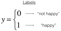
• Given:
  • 600 RGB (labeled) training images each of size 64×64, with labels 0 (not happy) and 1 (happy).
  • 150 (unlabeled) test images (also the ground-truths separately).
• Train a deep convolution neural net model for binary classification.
• Use the model to predict the labels of the test images and evaluate the model using the ground truth.

 

Details of the “Happy” dataset:

Images are of shape (64,64,3)
Training: 600 pictures

Test: 150 pictures

It is now time to solve the “Happy” Challenge.

We need to start by loading the following required packages.

import numpy as np
from keras import layers
from keras.layers import Input, Dense, Activation, ZeroPadding2D, BatchNormalization, Flatten, Conv2D
from keras.layers import AveragePooling2D, MaxPooling2D, Dropout, GlobalMaxPooling2D, GlobalAveragePooling2D
from keras.models import Model
from keras.preprocessing import image
from keras.utils import layer_utils
from keras.utils.data_utils import get_file
from keras.applications.imagenet_utils import preprocess_input
from keras.utils.vis_utils import model_to_dot
from keras.utils import plot_model
import keras.backend as K
K.set_image_data_format(‘channels_last’)
import matplotlib.pyplot as plt
from matplotlib.pyplot import imshow

Then let’s normalize and load the dataset.

X_train_orig, Y_train_orig, X_test_orig, Y_test_orig, classes = load_dataset()

​# Normalize image vectors
X_train = X_train_orig/255.
X_test = X_test_orig/255.

# Reshape
Y_train = Y_train_orig.T
Y_test = Y_test_orig.T

print (“number of training examples = ” + str(X_train.shape[0]))
print (“number of test examples = ” + str(X_test.shape[0]))
print (“X_train shape: ” + str(X_train.shape))
print (“Y_train shape: ” + str(Y_train.shape))
print (“X_test shape: ” + str(X_test.shape))
print (“Y_test shape: ” + str(Y_test.shape))

number of training examples = 600
number of test examples = 150
X_train shape: (600, 64, 64, 3)
Y_train shape: (600, 1)
X_test shape: (150, 64, 64, 3)
Y_test shape: (150, 1)

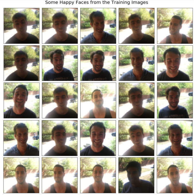
Now let’s find the number of labeled happy and unhappy faces in the training dataset.

print(X_train[Y_train.ravel()==1].shape, X_train[Y_train.ravel()==0].shape)

(300, 64, 64, 3) (300, 64, 64, 3)

As can be seen, there are equal numbers of positive and negative examples in the training dataset. The following figures show a few samples drawn from each class.

Building a model in Keras

Keras is very good for rapid prototyping. In just a short time we shall be able to build a model that achieves outstanding results.

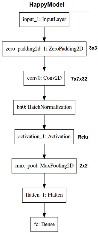
Let’s Implement a HappyModel() with the following architecture:

def HappyModel(input_shape):
“””
Implementation of the HappyModel.

Arguments:
input_shape — shape of the images of the dataset

Returns:
model — a Model() instance in Keras
“””

# Define the input placeholder as a tensor with shape input_shape. Think of
# this as our input image!
X_input = Input(input_shape)

# Zero-Padding: pads the border of X_input with zeroes
X = ZeroPadding2D((3, 3))(X_input)

# CONV -> BN -> RELU Block applied to X
X = Conv2D(32, (7, 7), strides = (1, 1), name = ‘conv0’)(X)
X = BatchNormalization(axis = 3, name = ‘bn0’)(X)
X = Activation(‘relu’)(X)

# MAXPOOL
X = MaxPooling2D((2, 2), name=’max_pool’)(X)

# FLATTEN X (means convert it to a vector) + FULLYCONNECTED
X = Flatten()(X)
X = Dense(1, activation=’sigmoid’, name=’fc’)(X)

# Create model. This creates our Keras model instance, you’ll use this instance
# to train/test the model.
model = Model(inputs = X_input, outputs = X, name=’HappyModel’)

return model

Step 1: Let’s first create the model.

happyModel = HappyModel((64,64,3))

Step 2:  Compile the model to configure the learning process, keeping in view that the Happy Challenge is a binary classification problem.

happyModel.compile(optimizer = “Adam”, loss = “binary_crossentropy”, metrics = [“accuracy”])

Step 3: Train the model. Choose the number of epochs and the batch size.

happyModel.fit(x = X_train, y = Y_train, epochs = 20, batch_size = 32)

Epoch 1/20
600/600 [==============================] – 6s – loss: 1.0961 – acc: 0.6750
Epoch 2/20
600/600 [==============================] – 7s – loss: 0.4198 – acc: 0.8250
Epoch 3/20
600/600 [==============================] – 8s – loss: 0.1933 – acc: 0.9250
Epoch 4/20
600/600 [==============================] – 7s – loss: 0.1165 – acc: 0.9567
Epoch 5/20
600/600 [==============================] – 6s – loss: 0.1224 – acc: 0.9500
Epoch 6/20
600/600 [==============================] – 6s – loss: 0.0970 – acc: 0.9667
Epoch 7/20
600/600 [==============================] – 7s – loss: 0.0639 – acc: 0.9850
Epoch 8/20
600/600 [==============================] – 7s – loss: 0.0841 – acc: 0.9700
Epoch 9/20
600/600 [==============================] – 8s – loss: 0.0934 – acc: 0.9733
Epoch 10/20
600/600 [==============================] – 7s – loss: 0.0677 – acc: 0.9767
Epoch 11/20
600/600 [==============================] – 6s – loss: 0.0705 – acc: 0.9650
Epoch 12/20
600/600 [==============================] – 7s – loss: 0.0548 – acc: 0.9783
Epoch 13/20
600/600 [==============================] – 7s – loss: 0.0533 – acc: 0.9800
Epoch 14/20
600/600 [==============================] – 7s – loss: 0.0517 – acc: 0.9850
Epoch 15/20
600/600 [==============================] – 7s – loss: 0.0665 – acc: 0.9750
Epoch 16/20
600/600 [==============================] – 7s – loss: 0.0273 – acc: 0.9917
Epoch 17/20
600/600 [==============================] – 7s – loss: 0.0291 – acc: 0.9933
Epoch 18/20
600/600 [==============================] – 6s – loss: 0.0245 – acc: 0.9917
Epoch 19/20
600/600 [==============================] – 7s – loss: 0.0376 – acc: 0.9883
Epoch 20/20
600/600 [==============================] – 7s – loss: 0.0440 – acc: 0.9917

Note that if we run fit() again, the model will continue to train with the parameters it has already learnt instead of re-initializing them.

Step 4: Test/evaluate the model.

preds = happyModel.evaluate(x = X_test, y = Y_test)
print()
print (“Loss = ” + str(preds[0]))
print (“Test Accuracy = ” + str(preds[1]))

150/150 [==============================] – 0s

Loss = 0.167731122573
Test Accuracy = 0.94666667064

As can be seen, our model gets around 95% test accuracy in 20 epochs (and 99% train accuracy).

Test with my own image

Let’s test on my own image to see how well the model generalizes on unseen face images.

img_path = ‘me_happy.png’
img = image.load_img(img_path, target_size=(64, 64))
imshow(img)

x = image.img_to_array(img)
x = np.expand_dims(x, axis=0)
x = preprocess_input(x)
print(happyModel.predict(x))

[[ 1.]]             # Happy !

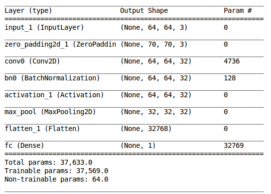
Model Summary

happyModel.summary()

 

2.  Face Recognition with Deep Neural Net

Face recognition problems commonly fall into two categories:

1. Face Verification – “is this the claimed person?”. For example, at some airports, one can pass through customs by letting a system scan your passport and then verifying that he (the person carrying the passport) is the correct person. A mobile phone that unlocks using our face is also using face verification. This is a 1:1 matching problem.
2. Face Recognition – “who is this person?”. For example, this video of Baidu employees entering the office without needing to otherwise identify themselves is an example of face recognition. This is a 1:K matching problem.

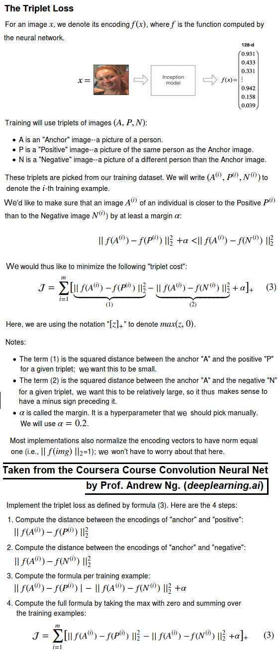
FaceNet learns a neural network that encodes a face image into a vector of 128 numbers. By comparing two such vectors, we can then determine if two pictures are of the same person.

In this assignment, we shall:

• Implement the triplet loss function
• Use a pretrained model to map face images into 128-dimensional encodings
• Use these encodings to perform face verification and face recognition

In this exercise, we will be using a pre-trained model which represents ConvNet activations using a “channels first” convention, as opposed to the “channels last” convention.

In other words, a batch of images will be of shape (m,n_C,n_H,n_W) instead of (m,n_H,n_W,n_C). Both of these conventions have a reasonable amount of traction among open-source implementations; there isn’t a uniform standard yet within the deep learning community.

Naive Face Verification

In Face Verification, we’re given two images and we have to tell if they are of the same person. The simplest way to do this is to compare the two images pixel-by-pixel. If the distance between the raw images are less than a chosen threshold, it may be the same person!

Of course, this algorithm performs really poorly, since the pixel values change dramatically due to variations in lighting, orientation of the person’s face, even minor changes in head position, and so on.

We’ll see that rather than using the raw image, we can learn an encoding f(img) so that element-wise comparisons of this encoding gives more accurate judgments as to whether two pictures are of the same person.

Encoding face images into a 128-dimensional vector

Using an ConvNet to compute encodings

The FaceNet model takes a lot of data and a long time to train. So following common practice in applied deep learning settings, let’s just load weights that someone else has already trained. The network architecture follows the Inception model from Szegedy et al.. We are going to use an inception network implementation.

This network uses 96×96 dimensional RGB images as its input. Specifically, inputs a face image (or batch of m face images) as a tensor of shape (m,nC,nH,nW)=(m,3,96,96).
It outputs a matrix of shape (m,128) that encodes each input face image into a 128-dimensional vector.

Let’s create the model for face images.

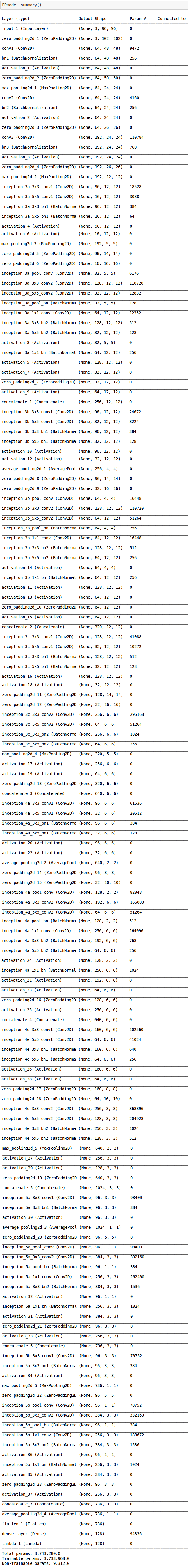
FRmodel = faceRecoModel(input_shape=(3, 96, 96))
print(“Total Params:”, FRmodel.count_params())

Total Params: 3743280

By using a 128-neuron fully connected layer as its last layer, the model ensures that the output is an encoding vector of size 128. We then use the encodings the compare two face images as follows:

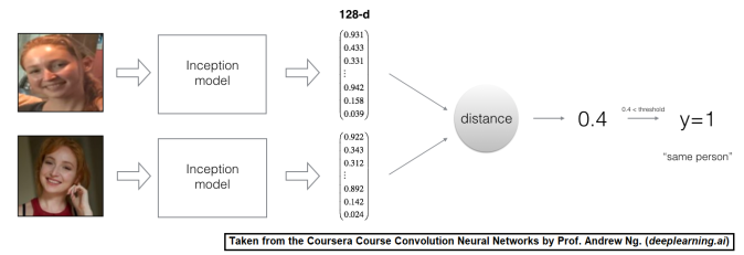
By computing a distance between two encodings and thresholding, we can determine if the two pictures represent the same person.

So, an encoding is a good one if:

• The encodings of two images of the same person are quite similar to each other
• The encodings of two images of different persons are very different

The triplet loss function formalizes this, and tries to “push” the encodings of two images of the same person (Anchor and Positive) closer together, while “pulling” the encodings of two images of different persons (Anchor, Negative) further apart.

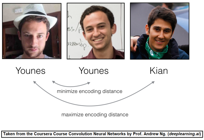
In the next part, we will call the pictures from left to right: Anchor (A), Positive (P), Negative (N).

 

Loading the trained model

FaceNet is trained by minimizing the triplet loss. But since training requires a lot of data and a lot of computation, we won’t train it from scratch here. Instead, we load a previously trained model. Let’s Load a model using the following code; this might take a couple of minutes to run.

FRmodel.compile(optimizer = ‘adam’, loss = triplet_loss, metrics = [‘accuracy’])
load_weights_from_FaceNet(FRmodel)

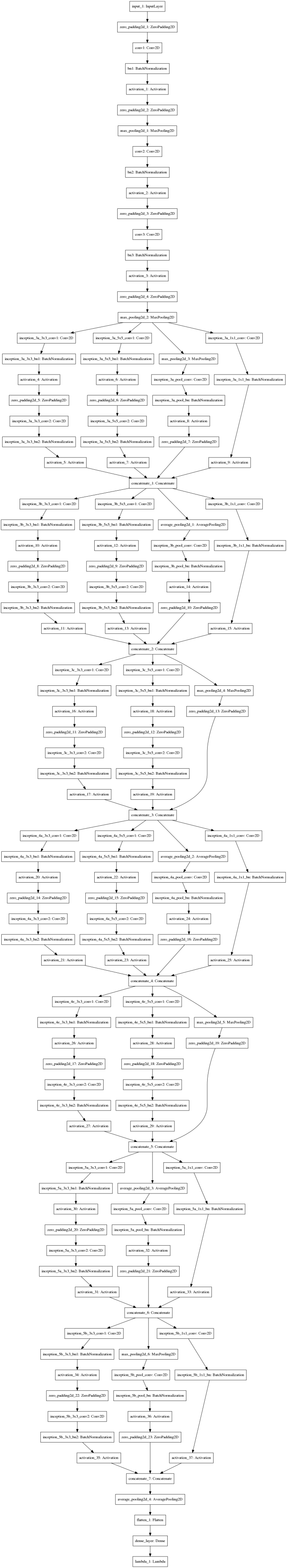
Here is the summary of the very deep inception network:

The next figure shows how the pre-trained deep inception network looks like:

Here’re some examples of distances between the encodings between three individuals:

Let’s now use this model to perform face verification and face recognition!

Applying the model

Face Verification

Let’s build a database containing one encoding vector for each person. To generate the encoding we use img_to_encoding(image_path, model) which basically runs the forward propagation of the model on the specified image.

Let’s build a database to map each person’s name to a 128-dimensional encoding of their face.

Now this can be used in an automated employee verification at the gate in an office in the following way: when someone shows up at the front door and swipes their ID card (thus giving us their name), we can look up their encoding in the database, and use it to check if the person standing at the front door matches the name on the ID.

Let’s implement the verify() function which checks if the front-door camera picture (image_path) is actually the person called “identity“. We shall have to go through the following steps:

• Compute the encoding of the image from image_path
• Compute the distance in between this encoding and the encoding of the identity image stored in the database
• Open the door if the distance is less than the threshold  0.7, else do not open.

As presented above, we are going to use the L2 distance (np.linalg.norm).

def verify(image_path, identity, database, model):

“””
Function that verifies if the person on the “image_path” image is “identity”.

Arguments:

image_path — path to an image

identity — string, name of the person you’d like to verify the identity. Has to be a resident of the Happy house.

database — python dictionary mapping names of allowed people’s names (strings) to their encodings (vectors).

model — your Inception model instance in Keras

Returns:

dist — distance between the image_path and the image of “identity” in the database.
door_open — True, if the door should open. False otherwise.

“””

### CODE HERE ###

return dist, door_open

Younes is trying to enter the  and the camera takes a picture of him (“camera_0.jpg”). Let’s run the above verification algorithm on this picture and compare with the one stored in the system (image_path):

verify(“camera_0.jpg”, “younes”, database, FRmodel)

# output
It’s younes, welcome home!
(0.67291224, True)

Benoit, has been banned from the office and removed from the database. He stole Kian’s ID card and came back to the house to try to present himself as Kian. The front-door camera took a picture of Benoit (“camera_2.jpg). Let’s run the verification algorithm to check if benoit can enter.

verify(“camera_2.jpg”, “kian”, database, FRmodel)

# output
It’s not kian, please go away
(0.86543155, False)

Face Recognition

In this case, we need to implement a face recognition system that takes as input an image, and figures out if it is one of the authorized persons (and if so, who). Unlike the previous face verification system, we will no longer get a person’s name as another input.

Implement who_is_it(). We shall have to go through the following steps:

• Compute the target encoding of the image from image_path
• Find the encoding from the database that has smallest distance with the target encoding.
• Initialize the min_dist variable to a large enough number (100). It will help to keep track of what is the closest encoding to the input’s encoding.
• Loop over the database dictionary’s names and encodings. To loop use for (name, db_enc) in database.items().
• Compute L2 distance between the target “encoding” and the current “encoding” from the database.
• If this distance is less than the min_dist, then set min_dist to dist, and identity to name.

 

def who_is_it(image_path, database, model):
“””
Implements face recognition for the happy house by finding who is the person on the image_path image.

Arguments:
image_path — path to an image
database — database containing image encodings along with the name of the person on the image
model — your Inception model instance in Keras

Returns:
min_dist — the minimum distance between image_path encoding and the encodings from the database
identity — string, the name prediction for the person on image_path
“””

###  CODE HERE ###

return min_dist, identity

Younes is at the front-door and the camera takes a picture of him (“camera_0.jpg”). Let’s see if our who_it_is() algorithm identifies Younes.

who_is_it(“camera_0.jpg”, database, FRmodel)

# output
it’s younes, the distance is 0.672912
(0.67291224, ‘younes’)

We can change “camera_0.jpg” (picture of younes) to “camera_1.jpg” (picture of bertrand) and see the result.

who_is_it(“camera_1.jpg”, database, FRmodel)

# output
it’s bertrand, the distance is 0.474829
(0.47482917, ‘bertrand’)

Here is the takeaway:

• Face verification solves an easier 1:1 matching problem; face recognition addresses a harder 1:K matching problem.
• The triplet loss is an effective loss function for training a neural network to learn an encoding of a face image.
• The same encoding can be used for verification and recognition. Measuring distances between two images’ encodings allows you to determine whether they are pictures of the same person.

 

References:

• Florian Schroff, Dmitry Kalenichenko, James Philbin (2015). FaceNet: A Unified Embedding for Face Recognition and Clustering
• Yaniv Taigman, Ming Yang, Marc’Aurelio Ranzato, Lior Wolf (2014). DeepFace: Closing the gap to human-level performance in face verification
• The pretrained model we use is inspired by Victor Sy Wang’s implementation and was loaded using his code: https://github.com/iwantooxxoox/Keras-OpenFace.
• Implementation by Ng. et al. also took a lot of inspiration from the official FaceNet github repository: https://github.com/davidsandberg/facenet