


The YOLO (You Only Look Once) series of models, renowned for its real-time object detection capabilities, owes much of its effectiveness to its specialized loss functions. In this article, we delve into the various YOLO loss function integral to YOLO’s evolution, focusing on their implementation in PyTorch. Our aim is to provide a clear, technical understanding of these functions, which are crucial for optimizing model training and performance.
By exploring the code behind these functions, readers can gain practical insights for their own deep learning projects, enhancing their ability to develop advanced object detection models. Specifically, we will review the Focal Loss and SIoU Loss used in YOLOv6 and YOLOv8. In the next part we will discuss Distribution Focal Loss (DFL) and Varifocal Loss(VFL).
Importance of Loss Functions
“Deep Learning training is a non-convex optimization problem.”
Let’s break this statement down. Deep Learning models are often regarded as a high dimensional mapping function, which takes some value as input and spits out a prediction. To understand if the prediction is right or wrong, we use a Loss function or Cost Function. This is nothing but a mathematical function to evaluate how far off the prediction is from the original value. Then the estimated loss is used to update the model parameters using an optimizer such as Stochastic Gradient Descent or adaptive moment estimation (ADAM). Typically, loss functions are categorized into two types: convex loss and non-convex loss functions. Both are discussed below.

Convex Function
Based on geometric representations, a convex function is defined as follows:
If you create a line by choosing any two distinct points from the graph of the function, and that line doesn’t have any intersecting points on the graph itself, then it can be regarded as a convex function. One unique property of a convex function is that it has only one global minima.
Examples: Mean squared error (MSE), Hinge loss, Cross Entropy loss etc. are examples of a Convex loss function.

Figure 1: Convex and Non-Convex Loss Function
Non-Convex Function
A Non-Convex Function is exactly the opposite of a Convex Function,
If the line created by two distinct points on the graph has intersecting points on the graph itself, then it is called a Non-Convex Function.
A non-convex function generally has multiple local minima, making it harder to optimize.
Examples: Triplet loss, Negative Log Likelihood with softmax activation etc.
YOLO Loss Functions
Loss functions in YOLO are of two types: classification loss and regression loss. The only exception is the YOLOv1, where the problem of object detection was formulated as a regression problem. Till YOLOv3, the losses were Squared loss for bounding box regression and Cross Entropy Loss for object classification. But, from YOLOv4, researchers started focusing more on the IoU-based losses, as it was a better estimate of bounding box localization accuracy.
More specifically, YOLOv5, YOLOv4, YOLOR and YOLOv7 authors used CIoU (Complete IOU) loss for their bounding box regression loss. In YOLOX, authors decided to go for normal IoU loss, YOLOv6 employs SIoU/GIoU as regression loss and VariFocal loss for classification task, CIoU and Distribution Focal Loss (DFL) loss functions being used for YOLOv8 bounding box loss. IoU Loss Functions for Object Detection is a great resource for understanding IoU, CIoU, DIoU, and GIoU loss functions in detail.
YOLO series of models are the state-of-the-art object detection models, which makes it more important to learning about the different YOLO models available. YOLOv5 custom training is a very comprehensive resource that talks about YOLOv5 training on custom dataset. Paper explanation for YOLOv6 has also been discussed here. YOLOv8 is one of the most important models in the YOLO series, in the following article we discussed about the YOLOv8 custom model training in-depth.
SCYLLA IoU (SIoU) Loss
SIoU is a unique loss function that involves four different cost functions such as,
- Angle cost
- Distance cost
- Shape cost
- IoU cost
When using Convolution based architectures, it was shown that SIoU improves both the speed of training and model accuracy. The author claimed directionality as the main reason for these improvements. Following is the in-depth explanation of each of the SIoU loss functions,
Angle Cost:
This is the angle-aware loss function part that helps improve training speed and accuracy. It helps to reduce the model complexity, specifically addressing the issue of “wandering” when predicting the distance-related variables. Here, “wandering” refers to the problem of varying bounding box prediction.Having too many degrees of freedom might cause this issue. DoF is defined as the number of basic ways you can move a rigid object in 3D space. Let’s look at some examples to understand the degree of freedom(DoF). What’s the DoF of a rigid body in 3D space? It has 6 DoF: x,y,z, roll(X-axis rotation angle), pitch(Y-axis rotation angle), and yaw(Z-axis rotation angle). Similarly, a 2D bounding box has 4 DoF, x,y (for center point) and width(w) and height(h) of the bounding box. The formula for angle cost is,

Figure a,b: (a) Angle Cost Formula; (b) Angle Cost Intuition Diagram
Given the predicted and ground truth box, the angle between the horizontal axis and the line joining the centers of each box is considered as  , and the angle with the vertical axis is taken as
  .
.  is the vertical distance between the centers of the two bounding boxes. The above loss function resembles a trigonometry formula,
 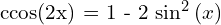 . The cost utilizes both and , model tries to minimize if
  otherwise it minimizes , where
  .
.
Distance Cost:
Distance Cost is designed taking angle cost into account. As the  the contribution of distance loss decreases drastically. Motivation for introducing the distance cost was to make the predicted bounding boxes fall near the ground truth bounding boxes. The paper says,
“So the 𝛾 was given time priority to the distance value as the angle increases.”
In other words, smaller angles of deviation between the predicted and actual bounding box might be considered less severe, while larger angles of deviation are penalized more.

Figure c, d: (c) Distance Cost Formula; (d) Distance Cost Diagram
Where,
 ,
,  = x coordinate of the ground truth and predicted bounding box,
 ,
,  = y coordinate of the ground truth and predicted bounding box
 ,
,  = smallest enclosing box or “convex box‘ width and height respectively,
and has been annotated in the figure d.
Shape Cost:
Shape Cost is the part that takes care of the aspect ratio mismatch. It is defined as,

Figure e,f: (e) Shape Cost Formula; (f) Shape Cost Diagram
Where,
 and
and  = the width of the predicted and ground truth bounding box,
 and
and  = the height of the predicted and ground truth bounding box, respectively.
 and
and  = relative difference in width and height between the two bounding boxes.
IoU Cost:
IoU cost is the normal intersection over union value subtracted by 1. Subtracting the IoU value by 1, emphasizes the non-overlapping part of the predicted bounding box.

Figure: IoU Cost Formula
The SIoU loss is defined using the Distance Cost, Shape Cost, and IoU Cost. The Angle Cost is utilized in the Distance Cost. Following is the SIoU formula,

Figure g: SIoU Formula
💡 You can access the entire codebase for this and all our other posts by simply subscribing to the blog post, and we’ll send you the link to download link.

SIoU PyTorch Implementation:
import torch
import torch.nn as nn
import numpy as np


class SIoU(nn.Module):
    # SIoU Loss https://arxiv.org/pdf/2205.12740.pdf
   def __init__(self, x1y1x2y2=True, eps=1e-7):
     super(SIoU, self).__init__()
     self.x1y1x2y2 = x1y1x2y2
     self.eps = eps


   def forward(self, box1, box2):


       # Get the coordinates of bounding boxes
       if self.x1y1x2y2:  # x1, y1, x2, y2 = box1
           b1_x1, b1_y1, b1_x2, b1_y2 = box1[0], box1[1], box1[2], box1[3]
           b2_x1, b2_y1, b2_x2, b2_y2 = box2[0], box2[1], box2[2], box2[3]
       else:  # transform from xywh to xyxy
           b1_x1, b1_x2 = box1[0] - box1[2] / 2, box1[0] + box1[2] / 2
           b1_y1, b1_y2 = box1[1] - box1[3] / 2, box1[1] + box1[3] / 2
           b2_x1, b2_x2 = box2[0] - box2[2] / 2, box2[0] + box2[2] / 2
           b2_y1, b2_y2 = box2[1] - box2[3] / 2, box2[1] + box2[3] / 2


       # Intersection area
       inter = (torch.min(b1_x2, b2_x2) - torch.max(b1_x1, b2_x1)).clamp(0) * \
               (torch.min(b1_y2, b2_y2) - torch.max(b1_y1, b2_y1)).clamp(0)


       # Union Area
       w1, h1 = b1_x2 - b1_x1, b1_y2 - b1_y1 + self.eps
       w2, h2 = b2_x2 - b2_x1, b2_y2 - b2_y1 + self.eps
       union = w1 * h1 + w2 * h2 - inter + self.eps

       # IoU value of the bounding boxes
       iou = inter / union
       cw = torch.max(b1_x2, b2_x2) - torch.min(b1_x1, b2_x1)  # convex (smallest enclosing box) width
       ch = torch.max(b1_y2, b2_y2) - torch.min(b1_y1, b2_y1)  # convex height
       s_cw = (b2_x1 + b2_x2 - b1_x1 - b1_x2) * 0.5
       s_ch = (b2_y1 + b2_y2 - b1_y1 - b1_y2) * 0.5
       sigma = torch.pow(s_cw ** 2 + s_ch ** 2, 0.5) + self.eps
       sin_alpha_1 = torch.abs(s_cw) / sigma
       sin_alpha_2 = torch.abs(s_ch) / sigma
       threshold = pow(2, 0.5) / 2
       sin_alpha = torch.where(sin_alpha_1 > threshold, sin_alpha_2, sin_alpha_1)

       # Angle Cost
       angle_cost = 1 - 2 * torch.pow( torch.sin(torch.arcsin(sin_alpha) - np.pi/4), 2)

       # Distance Cost
       rho_x = (s_cw / (cw + self.eps)) ** 2
       rho_y = (s_ch / (ch + self.eps)) ** 2
       gamma = 2 - angle_cost
       distance_cost = 2 - torch.exp(gamma * rho_x) - torch.exp(gamma * rho_y)

       # Shape Cost
       omiga_w = torch.abs(w1 - w2) / torch.max(w1, w2)
       omiga_h = torch.abs(h1 - h2) / torch.max(h1, h2)
       shape_cost = torch.pow(1 - torch.exp(-1 * omiga_w), 4) + torch.pow(1 - torch.exp(-1 * omiga_h), 4)
       return 1 - (iou + 0.5 * (distance_cost + shape_cost))
Code Explanation:
s_cwands_chcalculate the horizontal and vertical distances between the centers of the two bounding boxes (predicted and ground truth).sigmacomputes the Euclidean distance between the centers of the two boxes, with an added eps (a small value to prevent division by zero).sin_alpha_1andsin_alpha_2are and
and  respectively.
 thresholdis set to and if
 sin_alpha_1is greater than threshold then it is taken assin_alphaelsesin_alpha_2is set assin_alpha.- Using the
sin_alpha, angle cost is computed. rho_xandrho_ycompute normalized squared distances in width and height dimensions.gammais basically the angle cost subtracted from two.- Using this
gamma,rho_xandrho_ythe distance cost is calculated.omiga_wandomiga_hcalculate the relative difference in width and height between the two bounding boxes, and theta is set to four. - Later, the
shape_costis calculated as the exponential of the negativeomiga_wandomiga_h, raised to the fourth power. - Finally, the SIoU loss is computed utilizing the IoU cost, distance cost, and shape cost.
 and if
 Focal Loss:
Which loss function serves as the inspiration for the focal loss, binary cross entropy or categorical cross entropy? To answer this question let’s first explore the fundamentals of this loss function and how it helps in model training. We will circle back to this question at the end.
Focal loss was first introduced in 2017 in the paper named Focal Loss for Dense Object Detection by He et. al. It was the time when Object Detection used to be taken as a very hard problem especially if the dataset is imbalanced or objects to be detected are small. Following the lead from SSD, this paper tried tackling both problems simultaneously by introducing a unique model architecture named RetinaNet and a loss function named Focal loss.

Figure h: Focal Loss Formula
Figure h, shows the formula for focal loss, where , is the weighting factor,  is the modulating factor, and
  is the probability of the true class.
The previous generation of object detectors used to utilize cross entropy loss to solve the classification task. One trait of cross entropy is that it views things in binary, white and black, there is no gray in between. In other words, it praises the right predictions as much as it demeans a wrong prediction. This is mathematically true as well,

Figure: Binary Cross-Entropy and Categorical Cross-Entropy Loss Formula
Cross entropy is defined as the negative logarithm of probability . This means high probability and low loss. This is a good property for a loss function, giving equal weights to both positive and negative samples. However, below are scenarios where cross entropy fails to bring results,
- In case of class imbalance, the gradient calculated by the majority class contributes more to the loss function, causing the weights to update in the direction where it becomes easy for the model to detect the majority class. Because of the less contribution in the estimated loss by the minority class the it becomes harder for the model to predict them accurately.
- Difficulty in distinguishing between easy and hard examples. Easy examples are the data points on which the model makes fewer errors, and the hard examples are those on which the model makes huge errors frequently.
We have understood where cross-entropy fails, now let’s understand how focal loss was being formalized which helped solve the problems where cross entropy was failing. Most important bit to understand before proceeding with the formulation is the graph provided in the paper, which compares the cross-entropy loss with focal loss,

Figure i: Loss vs Probability plot of the Focal Loss Function
In Figure: i, the comparison between the loss values of binary cross entropy and focal loss for a specific probability value has been shown. We will observe two examples, one with low probability and one with high probability,
- In the case of p = 0.8, BCE Loss is near 0.2, and Focal Loss is near 0.0002.
- In the case of p = 0.2, BCE Loss is near 1.6 and Focal Loss is near 1.
Say there are 10 samples in a batch, and from those, 8 samples are from the majority class and 2 samples are from the minority class. Generally, the model will predict the majority class with a high probability(0.8) and the minority class with a low probability(0.2). In the case of focal loss, it dumps down the loss for the majority class more drastically compared to the minority class. In the case of the majority class, the loss goes from 0.2(CE) to 0.0002(FL), but in the case of the minority class, the loss goes from 1.6 (CE) to 1 (FL). For regulating the loss contribution of easy and hard examples, authors introduced the modulation factor . This property of focal loss solves the 2nd issue mentioned above(point 2).
A common method to address the problem of class imbalance is to add the weighting factor ![$\alpha \in [0, 1]$](https://learnopencv.com/wp-content/ql-cache/quicklatex.com-0dd14d05baf5032a022764804fef9ced_l3.png) for the true class, and (1 – ) otherwise. In practice, is set by inverse class frequency or treated as a hyperparameter to be set by cross validation. Before focal loss, a similar method was introduced in the balanced cross-entropy paper.
for the true class, and (1 – ) otherwise. In practice, is set by inverse class frequency or treated as a hyperparameter to be set by cross validation. Before focal loss, a similar method was introduced in the balanced cross-entropy paper.
Focal Loss PyTorch Implementation:
class FocalLoss(nn.Module):
    def __init__(self, alpha=None, gamma=2):
      super(FocalLoss, self).__init__()
      self.alpha = alpha
      self.gamma = gamma

    def forward(self, inputs, targets):
      p = torch.sigmoid(inputs)
      bce_loss = F.binary_cross_entropy_with_logits(inputs, targets, reduction='none')
      pt = p * targets + (1 - p) * (1 - targets)
      loss = (1 - pt) ** self.gamma * bce_loss
      if self.alpha>=0:
        alpha_t = self.alpha * targets + (1 - self.alpha) * (1 - targets)
        loss = alpha_t * loss
       loss = loss.mean()
      return loss

inputs = torch.randn(10)
targets = torch.randint(1, 5, (10,)).to(torch.float32)

loss = FocalLoss(alpha = 0.30)

print(loss(inputs, targets))
Code Explanation:
Basically, the focal loss is same as binary cross-entropy loss, with an added factor of  . A loss function defined in PyTorch is the same as how a model is defined, inheriting the
 nn.Module class. In the forward function, we first apply sigmoid to the logits to generate probability values(p). Next, we compute the binary cross entropy loss using the logits. Logits are simply the final raw model output, it represents the output before the last sigmoid or softmax layer.
The pt is the probability for the true class(positive class), which has been calculated as the p * targets + (1 - p) * (1 - targets), the (1-p) takes care of the negative samples. Utilizing the gamma, pt and bce_loss the loss is calculated. However, observe that the alpha part is missing from the loss calculation. alpha_t is also calculated in the similar fashion as p_t. Later this alpha is multiplied with the calculated loss, to get the balanced loss value. Remember, we pass the image and labels in a batch, so we need to average them to get a holistic representation of the loss for the entire batch.
The value of alpha can be computed as,
alpha_t = self.alpha * targets + (1 - self.alpha) * (1 - targets)
Here, a predefined value of alpha is provided, and the targets are the integer class labels. Below is an example of how the value of alpha is decided,
targets = torch.tensor([0.,0.,0.,0.,0.,1.,0.,0.,1.,0.])
alpha = 0.3
alpha_t = alpha * targets + (1 - alpha) * (1 - targets)
print(alpha_t) # output -> tensor([0.7000, 0.7000, 0.7000, 0.7000, 0.7000, 0.3000, 0.7000, 0.7000, 0.3000,0.7000])
Above, you can see that the estimated value of alpha is inverse class frequency constrained from 0 to 1.
Now, if we come back to the question, which loss function inspired the formulation of focal loss, binary cross-entropy or categorical cross entropy, it becomes evident that binary cross-entropy was the primary source of inspiration for the development of focal loss.
Key Takeaways:
- Loss Functions in Deep Learning: Loss functions are essential in deep learning to evaluate the difference between predicted values and actual values, guiding the optimization process.
- Convex vs. Non-Convex Loss Functions: Loss functions can be categorized into convex and non-convex types, with convex functions having a single global minimum, making them easier to optimize.
- Introduction to SIoU Loss: SIoU (Shape-Aware IoU) Loss is used in bounding box regression and takes into account aspects like shape, distance, and aspect ratio alignment for faster convergence and higher accuracy. SIoU Loss includes Angle Cost, Distance Cost, Shape Cost, and IoU Cost, which collectively contribute to a more precise bounding box localization.
- Focal Loss for Object Detection: Focal Loss addresses class imbalance problems in object detection models, emphasizing hard examples and effectively handling imbalanced datasets. Focal Loss improves upon Cross Entropy Loss by reducing the impact of majority class samples and distinguishing between easy and hard examples. Focal Loss allows for adjusting loss contribution with the parameter Alpha, which can be set based on inverse class frequency or as a hyperparameter.
- Use Cases: SIoU Loss and Focal Loss are widely used in deep learning models, especially in object detection, to enhance performance and address common challenges.
Conclusion:
Through the course of this article, we discussed the two YOLO loss function, SIoU Loss and Focal Loss. SIoU Loss is mostly used in bounding box regression. It is a IoU-based loss function for bounding box regression, which also takes shape, distance, and aspect ratio miss alignment into account. SIoU achieves faster convergence and higher inference accuracy than the existing methods. We also touched upon focal loss. Focal Loss is very powerful at handling class imbalance problems, and it is being used extensively when training object detection models.
Following these loss functions, a few others were introduced, such as Varifocal Loss (VFL) and Distribution Focal Loss(DFL), which are integrated with the YOLOv6 and YOLOv8, respectively. We will cover these two losses in the next part of the series YOLO Loss Function -Part 2. Stay tuned!
References:
[1] What is Focal Loss and when should you use it? by Aman Arora.
[2] SIoU Loss: More Powerful Learning for Bounding Box Regression by, Zhora Gevorgyan.
[3] Focal Loss for Dense Object Detection by Dollár et. al.
[5] Focal Loss code from pytorch.

