
Until now, you’ve probably expected all your tests to pass, but what happens when you test systems with inherent inbuilt randomness? AI is nondeterministic, which doesn’t cleanly fit within our current testing paradigms. Many tests may take the form of returning a number, such as time for speed testing or a percent for testing accuracy on an LLM. How to evaluate these results might not be clear, and that’s where statistics come in. You may think this will require you to run many tests, but this blog will give you a method for ensuring that we extract statistically valid results and how to do it quickly.
What is the t-test?
Testing for nondeterministic metrics such as speed or accuracy often involves running many tests. This can be time-consuming, and interpreting the results manually can be challenging. However, with the application of a simple statistical technique, we can expedite these tests and ensure that we are extracting statistically valid results.
We’ll start with the very basics of testing: what is a hypothesis test? In its simplest form, a hypothesis test has two parts: a null hypothesis and an alternative hypothesis. The null hypothesis is the hypothesis you are attempting to disprove, which is assumed true until proven otherwise, while the alternative hypothesis is the one you aim to prove.
The hypothesis test we will use is a t-test, specifically the dependent t-test. A t-test is used to compare the means of two related groups. This means you can use a t-test to assess the average performance of an LLM (Large Language Model) before and after a change to its architecture. In this case, the null hypothesis is that changes to the architecture have not affected the test results, while the alternative hypothesis suggests that the changes have led to a difference, be it positive or negative.
To do this, you need to gather two sets of data: one for the performance before the change and another for the performance of the LLM after the change. Ideally, you should be able to match the before and after data to each other on a test by test basis. This pairing is what makes the test we are doing the stronger “dependent” t-test.
Once you have gathered your data and specified your hypotheses, you can employ a statistical software package to conduct the t-test. The software package will compute a p-value, which represents the likelihood that the null hypothesis is true.
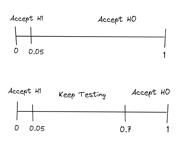
For a usual t-test, you would calculate your p-value after gathering all of your results. Then, if the value is less than a specific threshold (typically 0.05), you can reject the null hypothesis, H0, and conclude that there is a statistically significant difference in performance between the two groups. This is represented in the top diagram below. Depending on where you land on the line, it shows which hypothesis to accept. Given that our tests come at a cost, we will run our t-test after every result (or after small batches of results). If our p-value is more than 0.7, indicating the distributions are the same, or less than 0.05, indicating they are different, we will stop and accept the corresponding hypothesis. Essentially, we halt when we are reasonably certain that either our null hypothesis, H0, or alternative hypothesis, H1, is well-supported and continue otherwise. This is an exchange, you will lose some accuracy in exchange for speed.
Implementation
I will demonstrate how I implemented this in Jest, using this method to skip tests and this method to record results against tests for later use. A crucial aspect here is ensuring that each test can be matched with its previous result. While I’m implementing this in JavaScript, I hope the techniques are easily adaptable to other testing frameworks.
First, you’ll need to import a statistics module. This is infeasible without one, so you might as well choose one that does most of the work for you. I used statistics.js, but any general statistics module will contain a t-test.
Next, you must track your values as you run your tests. Here is where I employed the Jest snapshot matching technique described in the blog to store these values in the scoreArray.
it('First LLM Test', () => {
    const oldScore = fromSnapshot();
    const newScore = runModel();
    global.scoreArray.push({ before: oldScore, after: newScore });
    // assertions
});
Once we have stored our new and old scores as part of our test, we can perform the statistical test. First, we create a statistics object stats, and from here, we can perform many tests with the data provided. From this object, we call the t-test method studentsTTestTwoSamples. This comparison of the two groups returns the object taskSuccess with the pTwoSided property, which represents the p-value. As explained previously, a p-value of 0.05 indicates a 95% chance that the changes we made have resulted in a different set of results.
const minimumTests = 10;

skipIf(() => {
    if (scoreArray.length <= minimumTests) return false;

    const testVars = { before: 'interval', after: 'interval' };
    const stats = new Statistics(scoreArray, testVars);
    const taskSuccess = stats.studentsTTestTwoSamples('before', 'after', { dependent: true });

    return taskSuccess.pTwoSided > 0.7 || taskSuccess.pTwoSided < 0.05;
});
In the final step, we decide we are done if we are more than 95% confident that they are different or more than 30% confident that they are the same. These thresholds correspond to the confidence of each hypothesis. They can be configured where a higher upper bound increases the risk of falsely assuming they are different (type-1 errors), and a decrease in the lower bound increases the chance of falsely assuming they are the same (type-2 errors).
In the absence of a high probability for the alternate hypothesis, we default to the null hypothesis, which assumes that the two groups are the same.
You can also add a final test like this example. Negative t statistics indicate that the results are lower than expected, while positive t statistics suggest higher. So, this test will pass if the results are expected to be the same or better.
test('Have things not got worse', () => {
    expect(
        taskSuccess != null && taskSuccess.tStatistics <= 0 && taskSuccess.pTwoSided < 0.05
    ).toBe(false);
});
Assumptions and limitations of t-tests
However, it is important to note that dependent t-tests are based on certain assumptions. These assumptions include:
- The data is normally distributed.
- The data is continuous.
- The variances of the two groups are similar.
Luckily, most data with enough samples look normal. Two big things to watch out for are a lack of symmetry or expecting extreme values. Results taking the form of a percent will likely be normally distributed around the middle, but this becomes less true as you approach the 0 and 1 marks as the data gets less symmetrical. For example, coffee consumption is unlikely to be normal. These tend to have a right-skewed distribution, most values cluster around zero, with a few extreme values from heavy consumers to the right. If you’re worried about this, you can do the Shapiro–Wilks test or the Kolmogorov–Smirnov test on our data to check it is distributed normally.
The second assumption is that the data is continuous, but not really. The important part of this property comes from discrete data never being truly normal, but it can get pretty close. A t-test is quite robust, and given enough samples and data from a wide enough spread, discrete data can look normal. It should be fine if the data passes a normality test, but you may need to run more tests to meet this criterion. A test with a small possible set of results, like the results of a coin flip, will never look normal, no matter the number of results. In such cases, you can explore the use of Bernoulli trials to compare the results.
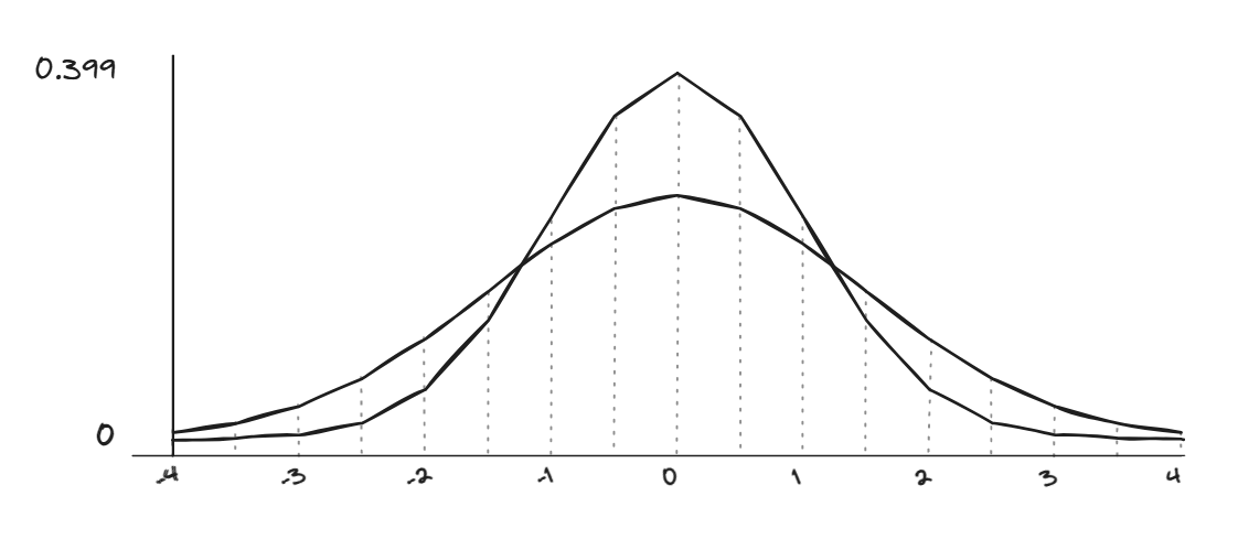
Our third assumption is that each distribution’s variance, the general spread, is the same. The t-test is only built to detect a difference in the mean. That means that for two distributions with means of 0, like in the graph below, the t-test would say they are the same. Therefore, they may not be suitable for detecting differences in properties like temperature variations as this will increase the spread of results while maintaining the same average. For these reasons, manually reviewing your test results may still be helpful.
The t-test is quite resilient, but if these assumptions are not met, then the results may be unreliable, and it’s important to keep these properties in mind.
Conclusion
This blog was about the t-test, but I hope it showed you how much you can do with only a little statistical knowledge. Using the t-test cleverly, you can speed up your testing process and ensure that you are still extracting provable statistical value. This can help you to identify meaningful changes in the performance of your LLM. However, it is important to be aware of the assumptions and limitations before starting.

