by Thalles Silva

How to deploy TensorFlow models to production using TF Serving

Introduction

Putting Machine Learning (ML) models to production has become a popular, recurrent topic. Many companies and frameworks offer different solutions that aim to tackle this issue.

To address this concern, Google released TensorFlow (TF) Serving in the hope of solving the problem of deploying ML models to production.

This piece offers a hands-on tutorial on serving a pre-trained Convolutional Semantic Segmentation Network. By the end of this article, you will be able to use TF Serving to deploy and make requests to a Deep CNN trained in TF. Also, I’ll present an overview of the main blocks of TF Serving, and I’ll discuss its APIs and how it all works.

One thing you will notice right away is that it requires very little code to actually serve a TF model. If you want to go along with the tutorial and run the example on your machine, follow it as is. But, if you only want to know about TensorFlow Serving, you can concentrate on the first two sections.

This piece emphasizes some of the work we are doing here at Daitan Group.

TensorFlow Serving Libraries — An Overview

Let’s take some time to understand how TF Serving handles the full life-cycle of serving ML models. Here, we’ll go over (at a high level) each of the main building blocks of TF Serving. The goal of this section is to provide a soft introduction to the TF Serving APIs. For an in-depth overview, please head to the TF Serving documentation page.

TensorFlow Serving is composed of a few abstractions. These abstractions implement APIs for different tasks. The most important ones are Servable, Loader, Source, and Manager. Let’s go over how they interact.

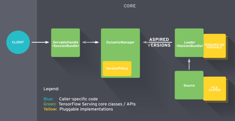
In a nutshell, the serving life-cycle starts when TF Serving identifies a model on disk. The Source component takes care of that. It is responsible for identifying new models that should be loaded. In practice, it keeps an eye on the file system to identify when a new model version arrives to the disk. When it sees a new version, it proceeds by creating a Loader for that specific version of the model.

In summary, the Loader knows almost everything about the model. It includes how to load it and how to estimate the model’s required resources, such as the requested RAM and GPU memory. The Loader has a pointer to the model on disk along with all the necessary meta-data for loading it. But there is a catch here: the Loader is not allowed to load the model just yet.

After creating the Loader, the Source sends it to the Manager as an Aspired Version.

Upon receiving the model’s Aspired Version, the Manager proceeds with the serving process. Here, there are two possibilities. One is that the first model version is pushed for deployment. In this situation, the Manager will make sure that the required resources are available. Once they are, the Manager gives the Loader permission to load the model.

The second is that we are pushing a new version of an existing model. In this case, the Manager has to consult the Version Policy plugin before going further. The Version Policy determines how the process of loading a new model version takes place.

Specifically, when loading a new version of a model, we can choose between preserving (1) availability or (2) resources. In the first case, we are interested in making sure our system is always available for incoming clients’ requests. We know that the Manager allows the Loader to instantiate the new graph with the new weights.

At this point, we have two model versions loaded at the same time. But the Manager unloads the older version only after loading is complete and it is safe to switch between models.

On the other hand, if we want to save resources by not having the extra buffer (for the new version), we can choose to preserve resources. It might be useful for very heavy models to have a little gap in availability, in exchange for saving memory.

At the end, when a client requests a handle for the model, the Manager returns a handle to the Servable.

With this overview, we are set to dive into a real-world application. In the next sections, we describe how to serve a Convolutional Neural Network (CNN) using TF Serving.

Exporting a Model for Serving

The first step to serve an ML model built in TensorFlow is to make sure it is in the right format. To do that, TensorFlow provides the SavedModel class.

SavedModel is the universal serialization format for TensorFlow models. If you are familiar with TF, you have probably used the TensorFlow Saver to persist your model’s variables.

The TensorFlow Saver provides functionalities to save/restore the model’s checkpoint files to/from disk. In fact, SavedModel wraps the TensorFlow Saver and it is meant to be the standard way of exporting TF models for serving.

The SavedModel object has some nice features.

First, it lets you save more than one meta-graph to a single SavedModel object. In other words, it allows us to have different graphs for different tasks.

For instance, suppose you just finished training your model. In most situations, to perform inference, your graph doesn’t need some training-specific operations. These ops might include the optimizer’s variables, learning rate scheduling tensors, extra pre-processing ops, and so on.

Moreover, you might want to serve a quantized version of a graph for mobile deployment.

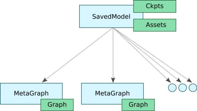
In this context, SavedModel allows you to save graphs with different configurations. In our example, we would have three different graphs with corresponding tags such as “training”, “inference”, and “mobile”. Also, these three graphs would all share the same set of variables — which emphasizes memory efficiency.

Not so long ago, when we wanted to deploy TF models on mobile devices, we needed to know the names of the input and output tensors for feeding and getting data to/from the model. This need forced programmers to search for the tensor they needed among all tensors of the graph. If the tensors were not properly named, the task could be very tedious.

To make things easier, SavedModel offers support for SignatureDefs. In summary, SignatureDefs define the signature of a computation supported by TensorFlow. It determines the proper input and output tensors for a computational graph. Simply put, with these signatures you can specify the exact nodes to use for input and output.

To use its built-in serving APIs, TF Serving requires models to include one or more SignatureDefs.

To create such signatures, we need to provide definitions for inputs, outputs, and the desired method name. Inputs and Outputs represent a mapping from string to TensorInfo objects (more on this latter). Here, we define the default tensors for feeding and receiving data to and from a graph. The method_name parameter targets one of the TF high-level serving APIs.

Currently, there are three serving APIs: Classification, Predict, and Regression. Each signature definition matches a specific RPC API. The Classification SegnatureDef is used for the Classify RPC API. The Predict SegnatureDef is used for the Predict RPC API, and on.

For the Classification signature, there must be an inputs tensor (to receive data) and at least one of two possible output tensors: classes and/or scores. The Regression SignatureDef requires exactly one tensor for input and another for output. Lastly, the Predict signature allows for a dynamic number of input and output tensors.

In addition, SavedModel supports assets storage for cases where ops initialization depends on external files. Also, it has mechanisms for clearing devices before creating the SavedModel.

Now, let’s see how can we do it in practice.

Setting up the environment

Before we begin, clone this TensorFlow DeepLab-v3 implementation from Github.

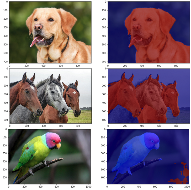
DeepLab is Google’s best semantic segmentation ConvNet. Basically, the network takes an image as input and outputs a mask-like image that separates certain objects from the background.

This version was trained on the Pascal VOC segmentation dataset. Thus, it can segment and recognize up to 20 classes. If you want to know more about Semantic Segmentation and DeepLab-v3, take a look at Diving into Deep Convolutional Semantic Segmentation Networks and Deeplab_V3.

All the files related to serving reside into: ./deeplab_v3/serving/. There, you will find two important files: deeplab_saved_model.py and deeplab_client.ipynb

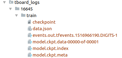
Before going further, make sure to download the Deeplab-v3 pre-trained model. Head to the GitHub repository above, click on the checkpoints link, and download the folder named 16645/.

In the end, you should have a folder named tboard_logs/ with the 16645/ folder placed inside it.

Now, we need to create two Python virtual environments. One for Python 3 and another for Python 2. For each env, make sure to install the necessary dependencies. You can find them in the serving_requirements.txt and client_requirements.txt files.

We need two Python envs because our model, DeepLab-v3, was developed under Python 3. However, the TensorFlow Serving Python API is only published for Python 2. Therefore, to export the model and run TF serving, we use the Python 3 env. For running the client code using the TF Serving python API, we use the PIP package (only available for Python 2).

Note that you can forgo the Python 2 env by using the Serving APIs from bazel. Refer to the TF Serving Instalation for more details.

With that step complete, let’s start with what really matters.

How to do it

To use SavedModel, TensorFlow provides an easy to use high-level utility class called SavedModelBuilder. The SavedModelBuilder class provides functionalities to save multiple meta graphs, associated variables, and assets.

Let’s go through a running example of how to export a Deep Segmentation CNN model for serving.

As mentioned above, to export the model, we use the SavedModelBuilder class. It will generate a SavedModel protocol buffer file along with the model’s variables and assets (if necessary).

Let’s dissect the code.

The SavedModelBuilder receives (as input) the directory where to save the model’s data. Here, the export_path variable is the concatenation of export_path_base and the model_version. As a result, different model versions will be saved in separate directories inside the export_path_base folder.

Let’s say we have a baseline version of our model in production, but we want to deploy a new version of it. We have improved our model’s accuracy and want to offer this new version to our clients.

To export a different version of the same graph, we can just set FLAGS.model_version to a higher integer value. Then a different folder (holding the new version of our model) will be created inside the export_path_base folder.

Now, we need to specify the input and output Tensors of our model. To do that, we use SignatureDefs. Signatures define what type of model we want to export. It provides a mapping from strings (logical Tensor names) to TensorInfo objects. The idea is that, instead of referencing the actual tensor names for input/output, clients can refer to the logical names defined by the signatures.

For serving a Semantic Segmentation CNN, we are going to create a Predict Signature. Note that the build_signature_def() function takes the mapping for input and output tensors as well as the desired API.

A SignatureDef requires specification of: inputs, outputs, and method name. Note that we expect three values for inputs — an image, and two more tensors specifying its dimensions (height and width). For the outputs, we defined just one outcome — the segmentation output mask.

Note that the strings ‘image’, ‘height’, ‘width’ and ‘segmentation_map’ are not tensors. Instead, they are logical names that refer to the actual tensors input_tensor, image_height_tensor, and image_width_tensor. Thus, they can be any unique string you like.

Also, the mappings in the SignatureDefs relates to TensorInfo protobuf objects, not actual tensors. To create TensorInfo objects, we use the utility function: tf.saved_model.utils.build_tensor_info(tensor).

That is it. Now we call the add_meta_graph_and_variables() function to build the SavedModel protocol buffer object . Then we run the save() method and it will persist a snapshot of our model to the disk containing the model’s variables and assets.

We can now run deeplab_saved_model.py to export our model.

If everything went well you will see the folder ./serving/versions/1. Note that the ‘1’ represents the current version of the model. Inside each version sub-directory, you will see the following files:

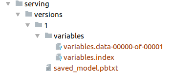
• saved_model.pb or saved_model.pbtxt. This is the serialized SavedModel file. It includes one or more graph definitions of the model, as well as the signature definitions.
• Variables. This folder contains the serialized variables of the graphs.

Now, we are ready to launching our model server. To do that, run:

$ tensorflow_model_server --port=9000 --model_name=deeplab --model_base_path=<full/path/to/serving/versions/>

The model_base_path refers to where the exported model was saved. Also, we do not specify the version folder in the path. The model versioning control is handled by TF Serving.

Generating Client Requests

The client code is very straightforward. Take a look at it in: deeplab_client.ipynb.

First, we read the image we want to send to the server and convert it to the right format.

Next, we create a gRPC stub. The stub allows us to call the remote server’s methods. To do that, we instantiate the beta_create_PredictionService_stub class of the prediction_service_pb2 module. At this point, the stub holds the necessary logic for calling remote procedures (from the server) as if they were local.

Now, we need to create and set the request object. Since our server implements the TensorFlow Predict API, we need to parse a Predict request. To issue a Predict request, first, we instantiate the PredictRequest class from the predict_pb2 module. We also need to specify the model_spec.name and model_spec.signature_name parameters. The name param is the ‘model_name’ argument that we defined when we launched the server. And the signature_name refers to the logical name assigned to the signature_def_map() parameter of the add_meta_graph() routine.

Next, we must supply the input data as defined in the server’s signature. Remember that, in the server, we defined a Predict API to expect an image as well as two scalars (the image’s height and width). To feed the input data into the request object, TensorFlow provides the utility tf.make_tensor_proto(). This method creates a TensorProto object from a numpy/Python object. We can use it to feed the image and its dimensions to the request object.

Looks like we are ready to call the server. To do that, we call the Predict() method (using the stub) and pass the request object as an argument.

For requests that return a single response, gRPC supports both: synchronous and asynchronous calls. Thus, if you want to do some work while the request is being processed, we could call Predict.future() instead of Predict().

Now we can fetch and enjoy the results.

Hope you liked this article. Thanks for reading!

If you want more, check out:

How to train your own FaceID ConvNet using TensorFlow Eager execution
Faces are everywhere — from photos and videos on social media websites, to consumer security applications like the…medium.freecodecamp.orgDiving into Deep Convolutional Semantic Segmentation Networks and Deeplab_V3
Deep Convolutional Neural Networks (DCNNs) have achieved remarkable success in various Computer Vision applications…medium.freecodecamp.org