
During my internship at Tweag, I got the opportunity to work on Chainsail (see the announcement blog post), a web service that helps to sample from multimodal probability distributions.
A common approach to sampling well-behaved distributions involves Markov chain Monte Carlo (MCMC) methods derived from the
basic Metropolis-Hastings algorithm; building a Markov chain that has the desired distribution as its stationary distribution.
The major benefit of Metropolis-Hastings over more “direct” sampling methods is that it doesn’t require the target distribution to be normalized.
But it does have a big flaw:
if the distribution presents multiple modes separated by areas of low probability, the Markov chain tends to get stuck in one mode, and thus samples the distribution incorrectly.
My work mainly consisted in improving Chainsail’s way of handling Bayesian data analysis problems.
Replica Exchange
Replica Exchange is an MCMC algorithm that allows us to overcome the problem of sampling multimodal distributions. You can find a detailed blog about RE here. Let’s consider a probability distribution with an unknown normalization constant. We can associate with an energy via
We then introduce different replicas
of our distribution, where is a sequence of values between 0 and 1, with being the target distribution. As seen in the figure, these values (or “inverse temperatures”) determine the “flatness” of each replica. At high temperatures () the low-probability regions are easily crossed, unlike in the original replica (). The high-temperature replicas are thus easier to sample since they don’t get stuck in one mode.
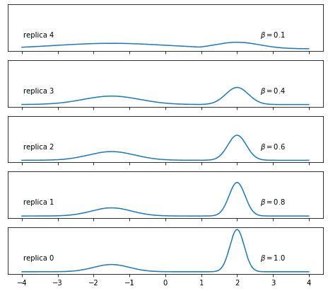
Five replicas of a Gaussian mixture distribution: in the flatter replicas, it’s easy to cross the region between the two “bells”
If we sample simultaneously from all the replicas, while performing every now and then an exchange between the states they reach, we can make sure to correctly sample to the original replica.
We have to make sure that the target replica () is participating sufficiently in the swap to be correctly sampled.
We can do so by allowing the exchange only between adjacent replicas.
A major challenge, however, in the algorithm is the choice of intermediate temperatures:
too little and we sample incorrectly due to the lack of flat distributions; too much and we waste computing time.
Replica Exchange scheme for Bayesian data analysis
With Bayesian methods becoming increasingly popular in data analysis, Chainsail ought to adapt. In this paragraph, we introduce a Bayesian Replica Exchange scheme, the implementation of which was my main task during the internship.
General theory
In Bayesian inference, we can construct a probability (or belief) distribution for parameters that we want to infer from some data . But it turns out that we also need to model the prior knowledge of our parameters, because, according to Bayes’s theorem, we have
where is the posterior and is the likelihood, that is, the probability of observing the data if the value of the unknown parameter is .
The prior encompasses our knowledge before having observed any data.
Habeck et al. 1 suggest an extended version of Monte-Carlo Replica Exchange for simulating the posterior density in a Bayesian Data analysis problem, by applying the inverse temperature parameter only to the likelihood.
This has the advantage of keeping the sampling fully informed by the prior distribution (which encodes established knowledge) instead of, for low inverse temperatures, exploring an essentially flat and uninformed parameter space.
More formally, they consider a family of distributions,
in which the inverse temperature weighs the likelihood and therefore determines the influence of the data. At , the data is fully taken into account, while at it is fully neglected. The exchange between replicas proceeds in the same way as in the basic Replica Exchange algorithm.
Implementation
Overview of relevant Chainsail components
Now that we have introduced the general theory of Replica Exchange and the Bayesian version of it, we can move to consider parts of the code of Chainsail. Chainsail is a Replica Exchange implementation with automated tuning and support for cloud computing platforms which provide the necessary parallel computing power. Its backend consists of several components, some of which needed to be adapted in order to implement the Bayesian Replica Exchange scheme, and we briefly present them in the following.
Runner : runs a Replica-Exchange simulation using Hamiltonian Monte Carlo with parameters provided in the job specification. We use a Message Passing Interface (MPI)-based runner to perform parallel sampling on multiple nodes. It’s also designed for use in high-performance computing.
Job specification : consists of a probability distribution and a range of parameters for the controller. These parameters include primarily the dependencies, the number of samples for both the optimization and the production, the maximum and initial number of nodes to be used, and the target acceptance rate. The job specification may also include parameters for local samples like the step size and the number of steps to perform in Hamiltonian Monte Carlo.
Controller : triggers multiple Replica Exchange simulations (executed by the runners) and, during each simulation, estimates the density of states using multiple histogram re-weighting (see below). Based on the density of states, it tries to improve the set of inverse temperatures until the desired acceptance rates are achieved. For the very first run, a naive inverse temperature schedule is used that follows a geometric progression. The first runs are only used to optimize the inverse temperature schedule. The last run is the production run and is performed with an optimized schedule and initial states.
Necessary code changes
A class that transforms the user-defined probability distribution into the tempered likelihood scheme already existed, but the rest of the Chainsail code was only designed for a Boltzmann family distribution type of Replica Exchange. I was asked to make the code more flexible to be able to accommodate both schemes during my internship. I first began by extending the job specification to allow both tempering schemes. The majority of the changes, however, were in the controller, and they are as follows:
-
As the controller’s role is to implement the main loop of a running simulation by optimizing the schedule, and determining new initial states for the next simulation, and then setting up and running the simulation; the interface had to be extended to allow both tempering schemes, since the Boltzmann tempered scheme was hardcoded.
-
The configuration template, which is a nested dictionary of the user-provided and sampling parameters that is later turned into a configuration file for the runner, was extended to include a key about the type of tempering scheme.
-
The function that returns optimisation objects (like the initial temperature schedule, the schedule optimizing algorithm and the Density of states estimation algorithm) had to be adapted as it was hardcoded for the Boltzmann tempered scheme.
Finally, the runner had to be enabled to read the type of tempering in use from the configuration file generated by the controller.
This concludes the coding-related part of my internship. Now I’ll move on to discuss a couple of other things that I learned when working on Chainsail and found interesting.
Related concepts and algorithms
Chainsail uses a couple of concepts and algorithms that might not be widely known among its intended audience. To gain a full understanding of how Chainsail works, an important part of my internship consisted in learning about these topics, which I briefly present in the following.
Density of states
When trying to optimize the acceptance rate and draw good initial states based on previous ones, one can use the concept of the density of states. This proves to be a computationally efficient approach, since it spares us from calculating multidimensional integrals. In this section, we introduce the density of states and, as an example of its application, show how it can be used to calculate the normalization constant of a probability distribution.
General theory
Let be the normalizing constant of an unnormalized distribution that can be defined through an energy . We note that can be written as
which is a potentially high-dimensional integral over the full parameter space and therefore costs a lot of computation time to estimate. A nice way to overcome this issue is to change the variables by defining the density of states
where is the Dirac delta function. The density of states quantifies the multiplicity of a given energy value over an interval . This is also difficult to calculate, but we will present an algorithm for that later in this post. Using the density of states, we can rewrite the normalization constant as
We can see that this second integral is one-dimensional as opposed to the first definition of . Therefore, if the density of states is available, the normalization constant is much easier to estimate. Let’s assume once again that , where is the normalization constant for the distribution at inverse temperature . This family of distributions uses a single energy function , and thus the normalizing constants are given by
With the density of states at our disposal, we can calculate the normalising constants for any . The following section details a method to estimate .
Weighted Histogram Analysis Method
The Weighted Histogram Analysis Method (WHAM) allows us to obtain an estimate for the density of states () from samples at different inverse temperatures.
We first discretize the energy in a histogram with a bin width of . For an inverse temperature , we denote with the value of the density of states where . If is the number of samples in bin and the total number of samples is , we can estimate as
But we can also estimate via the density of states by observing that the number of states with energy is and, via the previously defined energy-probability relation, the probability of a state with energy occurring is proportional to . This means that
Equating the right-hand sides of the last two equations allows us to derive
as an expression for the density of states , but it is not easily evaluated. Because of
the density of states equation is expanded to
and we observe that also appears non-trivially on the right hand side of the equation.
This equation has thus to be solved self-consistently, which can be done via a simple fixed point iteration algorithm.
Note that this estimation only uses samples from a simulation at a single temperature.
One can combine multiple estimates from different temperatures for better results2, however, that will involve multiple histogram reweighting.
A big inconvenience in what we just did is that we overlooked the correlation between samples.
To improve the formula above we could introduce a statistical inefficiency factor, which is the number of configurations after which we obtain uncorrelated samples.
Internship in the Tweag Paris office
Working at Tweag opened my eyes to many skills essential to data scientists and software engineers. An example of one of these skills is Git, which is a distributed, open-source version control system that enables developers to track code, merge changes and revert to older versions. It also enables teamwork by helping to avoid code conflicts while coding. On a different note, I had the chance, for the first time in my academic curriculum, to work continuously on a single project and be entirely immersed in it for three months straight.
Beside all the technical skills I’ve learned, I also had the chance to work in a professional environment for the first time in my life, allowing me to gain the ability to demonstrate initiative, be a team-player, as well as manage my time. It was immensely helpful to receive feedback and help whenever I needed them. I appreciated the fact that I was afforded the opportunity to take responsibility for a project, which provided me with a depth of knowledge I would not have gained in the classroom alone.
I particularly enjoyed working at the Tweag office in Paris, where there’s a great encouraging ambience. One of the best ways of building networks in the company, besides going together to have lunch, was a Slack channel that randomly pairs colleagues for a virtual coffee break.
Conclusion
Tweag is my first experience in a professional environment outside of classrooms. Although it was a short experience over the summer, I definitely enjoyed it to the fullest. I learned so many new things about Bayesian inference, Replica Exchange and Git. And I had fun getting to know to new people, including my mentor Simeon!


