Logic Through the Lens of Neural Networks

Recently, I was experimenting with building small neural networks for sequence-to-sequence use cases. My goal was to create a visualization of how the inner state of a RNN changes as it processes inputs - similar to the browser-based neural network visualization I built previously.
I was inspired to explore this area after reading a very interesting blog post called Differentiable Finite State Machines which gave an overview of using gradient descent to learn FSMs to operate on one-bit strings. The state machines that were learned by their approach were impressively concise and managed to find optimal solutions in many cases.
As I started to try out different ideas in this space, I quickly ended up getting pulled into several fascinating rabbit holes of related topics in math, computer science, and machine learning. There's a ton of research being done in areas that border the work that I ended up doing. Artificial neural networks serve as very useful proxies for studying topics such as computational complexity, information theory, and probability among others.
This post is a sort of chronicle of the findings and observations I've made during my experiments with neural networks and similar things. It explores the connections between some of these topics and how they apply to machine learning both in theory and in practice, and the huge degree of overlap that these topics have with each other as well.
Learning Logic with RNNs
For my own work, I wanted to try learning things that would be able to make better use of the greater power and generality of full-fledged neural networks such as functions with multiple inputs/outputs, logic circuits, and maybe even some text generation or signal generation.
RNNs are more than capable of doing all of these things, but I had a constraint of keeping the model small/simple enough that a visualization of it will be intelligible and have a discernable method of action rather than just appear as a random mass of blinking lights.
My initial trails were working quite well. After some tuning of hyperparameters like learning rate, optimizer, and activation function, I was able to pretty consistently train networks to solve very simple problems like out[i] = in[i - 1] or out[i] = in[i] && in[i - 1] and do so in the minimum number of parameters (layer counts and sizes) for the network architecture.
Here's an example of an RNN that correctly models out[i] = in[i] && in[i - 1]:
![A diagram showing the architecture of a recurrent neural network that models out[i] = in[i] && in[i - 1]. The flow of data and the operations applied to values are indicated by arrows and signs. It shows the weights, inputs, and outputs for two steps of a sequence.](https://cprimozic.b-cdn.net/static/350180304f3ea62d2bbfcd8e752e2211/160fe/very_basic_rnn.png)
The recurrent tree has learned to populate the next state with the current input. Since we're using a linear/identity activation function, all we have to do is set the weight to 1 for the input - passing it through exactly. The previous state is completely ignored by setting its weight to 0. This gives the neuron the following truth table:
| Input 1 | Input 2 | Output | Rounded Output |
|---|---|---|---|
| 0 | 0 | 0 | 0 |
| 1 | 0 | 1 | 1 |
| 0 | 1 | 0 | 0 |
| 1 | 1 | 1 | 1 |
The output tree also takes the current state and current input, passing the result to the current output. Since the outputs of our network can be any number - not just 0 and 1 like the inputs - we round values that are < 0.5 to 0 and >= 0.5 to 1. Our output neuron takes advantage of that fact by setting the weights for each of the inputs to 1/3. That produces the following truth table:
| Input 1 | Input 2 | Output | Rounded Output |
|---|---|---|---|
| 0 | 0 | 0 | 0 |
| 1 | 0 | 0.333 | 0 |
| 0 | 1 | 0.333 | 0 |
| 1 | 1 | 0.666 | 1 |
So the output neuron has modeled a binary AND gate! Given this architecture and parameter values, the network will always make correct classifications for all inputs, assuming they all consist of only ones and zeros.
So every different set of parameters that one of these neurons can take on has a truth table which represents its output given all possible inputs. This represents a "binarized" view of the neuron, and it leaves out a good deal if information. This is especially significant in situations with multiple layers, or in RNNs where neurons' output is fed back in as inputs.
In order to better understand the neuron's behavior, we can visualize its output space - a continuous view that shows the neuron's output at every point across its input range for a given set of parameters (weights and bias). Since these neurons have 2 inputs, this can be done by creating a 2D plot, assigning on each input to an axis, and sampling the neuron's output at each pixel to determine its decision. Each corner of the plot represents a different combination of binarized inputs, and the color at that corner represents the decision: red is false, and green is true.
Here's an output plot for the output tree neuron with the weights from earlier:
The tiny patch of bright red in the top left corner represents regions of the function where outputs are very nearly 0, close to perfectly representing the negative class. The white stripe is the decision boundary where the classification switches between negative and positive. The only green corner is at (1, 1), just like the truth table.
Linear Separability
Given the fact that our activation is linear/the identity function, this proves that the binary boolean AND function is linearly separable. The decision boundary is a single straight line that that separates the trues from the falses.
There are a total of 16 binary boolean functions. OR, NAND, and the simple ones like "constant true" can be created by tweaking the weight and bias params; give it a try with the sliders on the viz if you'd like.
As it turns out, 14/16 of them are linearly separable and can be solved by neurons that have no activation function (these are called perceptrons). The exception is XOR and its complement XNOR. This fact is widely known and is often featured in machine learning teaching material, where it is known as the "XOR Problem". In order for a perceptron-based neural network to model XOR, it needs to have multiple layers.
This is a fascinating idea to me. Why is XOR "harder" to compute than the other logic gates? Is it some consequence of the mathematical operations used to implemented artificial neurons, or something intrinsic with XOR or boolean logic itself? XOR's unique properties are often used in cryptography to encode information or in hash functions to compress/destroy it.
As I later learned, there is indeed something that makes XOR and XNOR special compared to the other 2-input boolean functions. We'll get to that later on though!
Another thing to note, is that although 14/16 of the functions can be linearly separated perfectly with no activation function, the solutions aren't perfect in that the values are exactly true or false at the corners. Some functions can be perfectly represented like NOT Y which is achievable by setting xWeight = 0, yWeight = -1, bias = 1. For most of the others, however, no perfect solution exists and the outputs will be inexact for at least some inputs.
Solving the XOR Problem
So far, we've been working without activation functions. What if we add one of those in?
Dozens of different activation functions have been used in artificial neural networks, and the ones which are most commonly used change over time. They have a wide range of origins in ML research and other areas of study like statistics and electronics. Despite that, most of them can't represent XOR.
In order to solve XOR, the function needs to have more than one linear decision boundary. One example of a type of function that has this property is called GCU, which stands for Growing Cosine Unit. It was found to be quite effective when used in image classification networks, improving both the speed at which the networks train as well their classification accuracy. Also, in the research paper presenting the function, the authors prominently state that it can solve the XOR problem in a single neuron.
GCU has a simple equation of y = x * cos(x):
Sine and cosine are examples of what's known as oscillatory functions - they cross over y=0 an infinite number of times. This property gives them more than one linear decision boundary, which if you remember is the part of the function where the classification switches between negative and positive.
This can be seen in its 2D neuron response plot:
As you can see above, the GCU activation function can indeed model an XOR gate in a single neuron! Even y = cos(x) as an activation function works just fine, too, but GCU has the benefit of preserving at least some of the information about the magnitude of input signals.
These functions do have some problems for my particular use case though. Although GCU and similar oscillatory functions can model all the logic gates, they do so with considerable error. GCU doesn't saturate, so there are only single points where it is equal to the target values. In addition, it is not bounded so both its maximum value and maximum derivative is infinite. This can make training larger neural networks more difficult and require workarounds like weight regularization to counteract.
Neural networks usually have many neurons in each layer, and have multiple layers. By combining signals from multiple neurons and refining them through the layers, ANNs can figure out ways to minimize this error or eliminate it entirely. However, if the activation function used by the individual neurons was more expressive and yielded clearer signals from the start, I figured that it might allow the networks to learn with less resources or in less training time.
Designing a New Activation Function
I wondered if it was possible to create an activation function that fixed all of these issues - perfectly modeling all of the 2-input boolean functions with zero error. I also wanted it to be as simple as possible so that it would work well for my RNN visualization and be efficient during training.
I knew that the function would need to change direction at least once so that it crossed the decision boundary at least two times - a requirement for modeling XOR. As a starting point, I used variations of simple functions like |x| which indeed solved the XOR problem but failed to model the others with low error.
Along the way, I realized that having the function saturate at the target classes made it much easier to represent solutions since there was more freedom in the parameter choices.
After some much trial and error, I developed a function which did the job:
This function (which I will refer to as the Ameo activation function for the remainder of this writeup) has several characteristics that make it capable of modeling all the functions perfectly and suitable for use in neural networks:
- It changes direction 2 times and crosses the decision boundary (y=0) three times. This allows it to model XOR and XNOR.
- It saturates at both the positive and the negative ends of its range - very useful for modeling AND and NAND.
- Both its range and derivative are finite which helps keep weights and gradients from getting too large.
- It crosses through the origin, meaning that an input of 0 outputs zero as well. This is useful when training networks and helps keep things numerically balanced.
- It is symmetrical across x=0 from x=[-∞,∞] and has an average output of 0 across that domain.
- It is very straightforward to implement as a piecewise function:
I don't know if there are simpler functions that work for modeling binary boolean functions gates in artificial neurons with zero error, but in any case this particular function has some additional properties that make it useful for additional tasks which I'll detail later on.
Improvements
The function did have some issues though:
- It had large regions on either side where the gradient is zero which makes it vulnerable to the Vanishing Gradient Problem.
- It had areas where it only touched the target values (y=-1 and y=1) at single points. This makes parameters that solve it perfectly more difficult to find.
To resolve these issues, I created a modified version of the Ameo function which is created out of scaled, shifted, and reflected segments of y = x^4 instead of y = x. I also changed it from having a gradient of 0 at its edges to being optionally "leaky" in the same way as the Leaky ReLU. The leakiness does introduce a very small amount of imprecision for some functions, though, but it is negligible.
This new version has the benefit of having much more of its range output values that are near the targets of -1 and 1. There are many more "almost exact" solutions available, and the gradients leading to them are steeper which makes learning faster.
It still had one new issue, though, which is that regions where the gradient was very close to 0 remained at some parts of the domain. This can cause gradient descent to get "stuck" at those points, slowing down learning. As a solution, I created a final version of the function which interpolates between the y=x^4 and y=x versions with a configurable mix factor:
Here's the 2D response plots for the different versions of the Ameo function:
The checkboxes in the truth table can be used to change the function modeled by the neuron, picking parameters for the weights + bias such that it does so with no error. One nice thing is that the parameter values for the solutions are identical between all the variants.
The Next Dimension
In addition to binary logic gates, I also wanted to implement programs that did things like conditionals and if/then logic. In programming, this would be represented by a conditional operator also known as a ternary:
a ? b : c
I got to wondering if the Ameo activation function would work for solving this and other 3-input boolean function cases as well. The function crosses the decision boundary three times which we know is the requirement for separating 3-dimensional functions. That being said, I didn't know whether this particular function would be able to do it.
In order to test the idea, I implemented the function in TensorFlow.JS, the JavaScript port of the massively popular TensorFlow machine learning library. Since the function is pretty simple, it wasn't horrifically difficult - plus I only bothered implementing a kernel for the CPU backend which is implemented in pure JS rather than the WebGL backend which is much more complicated.
There are 256 different unique 3-input boolean functions compared to 16 for the 2-input case, many more than I was willing to determine manually. So, I figured I'd do as the neural networks do and let gradient descent discover some solutions for me.
After testing out learning a few different 3-input boolean functions, it didn't take long for me to realize that all the solutions gravitated towards parameters with integer-valued weights just like the 2-input solutions. After that realization, I wrote a quick program to attempt to brute-force solutions.
Results
The Ameo activation function has lossless solutions for 224/256 of the 3-input boolean functions and can perfectly classify the 32 others with some small error.
These 224 functions with solutions do include the conditional a ? b : c which can be solved with parameters of x_weight: -1, y_weight: 3, z_weight: 2, bias: -1
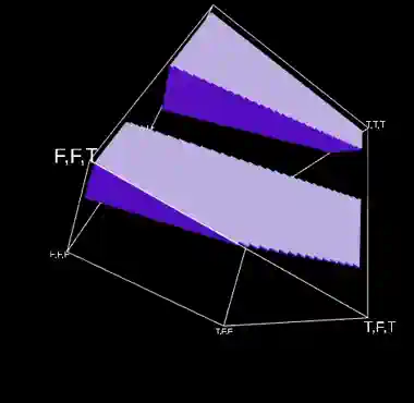
In order to visualize how the function achieves this solution, we can use the same approach as the 2D method of sampling the function at all points of its domain with a fixed set of parameters and measuring its output at many points in space - but we have to add a dimension to account for the added input:
You can click/drag to rotate the viz and use scroll wheel/pinch to zoom in and out. Filled regions of the cube represent a true output while empty regions are false. If you look at the labels at the edges, you'll see that the corners that are filled line up with the truth table for the conditional function.
To solve it, the function has wedged the positive "peak" of the function in at just the right angle such that it perfectly covers the TTF and FFT cases while leaving the FTF case exactly negative.
Playing with the parameters reveals that with the added input, the function can now be rotated in all three axes and the bias allows it to be shifted arbitrarily in any 3D direction. The decision boundaries are now planes rather than lines, and all three are apparent and indeed utilized to model the conditional. Notice, though, they're all still exactly parallel to each other and infinite.
For the 32 functions that aren't modeled perfectly, there exist non-perfect solutions with non-integer parameters that correctly classify all 8 input combinations with some error - meaning that they are non-zero and their sign matches the sign of the target.
An interesting thing I noticed is that the ratio of imperfectly modeled 3-input functions (32/256 = 1/8) is the same as the ratio of linearly inseparable 2-input functions (2/16 = 1/8).
The Ameo Activation Function in Practice
So although the Ameo activation function can indeed model all of the 3-input boolean functions, the question still remains of if (and how well) it can do so in practice. Given randomly initialized parameters and random inputs, can a neuron using the activation function actually learn effectively?
To test this, I used the same TensorFlow.JS setup I had created before to build a single neuron using the activation function and tested learning a variety of different functions. I wanted to see how long it took to find the various solutions and how reliably they were found compared to other activation functions that could also represent them.
The results were... somewhat difficult to ascertain. When training tiny models like this, the chosen hyperparameters for things like initial values for the parameters, learning rate, optimizer, variant of the Ameo activation function used, and even loss function have a huge impact on how well the learning performs.
I suspect that part of this is due to the Ameo activation function being a good bit more complex than many other activation functions. The fact that the gradient switches direction multiple times - a key feature providing it much of its expressive power - makes it harder for the optimizer to find valid solutions. Especially with low batch sizes or low learning rates, the function can get stuck at local minima.
The Adam optimizer helps combat this problem by keeping track of the "momentum" of the parameters being optimized. This can allow it to escape local minima by trading off some short-term pain in the form of increased loss for the reward of a lower loss at the other side.
In larger networks with many neurons and multiple layers, it becomes much easier for networks to learn. I don't have any proof or references for this, but I get the feeling that the reason is related to the birthday paradox. As the population of candidate starting parameters increases linearly, the probability of some particular combination of them existing in that population increases exponentially. Gradient descent is profoundly adept at locking onto those good combinations of parameters, maximizing their signal, and minimizing the noise to create good solutions.
Relationship to ML Theory
The optimizers used for training neural networks are very good at their job. They've been iterated on in research for decades and in general do an extremely good job of finding good solutions in the massive parameter space available.
However, the fact remains that some functions are just easier to learn than others. It is far easier to train a neural network to classify whether or not a given image consists of all black pixels than it is to train one to classify whether or not the image contains a human face.
Even in the domain of boolean functions, there are still some functions that are simply "harder" than others. Going back to the XOR problem, XOR and XNOR have some characteristic that just makes them more complex than the others. They're the only 2-input boolean functions that can't be linearly separated after all.
Boolean Complexity
One way of quantifying this is called Circuit Complexity, also known as Boolean Complexity. It assigns a complexity measure to boolean functions based on the minimum number of AND, OR, and NOT gates that are required to build a circuit representing it. There's a lot of CS theory that touches this subject, much of which is in the domain of computational complexity.
An alternative form of measuring boolean complexity ignores NOT gates and counts them as free. NOT gates are indeed "simpler" than an AND or OR gate since they only consider a single input rather than combining two input signals. For the rest of this writeup, I'll be referring to this measure as "AND/OR" complexity.
Using this measure of AND/OR complexity, it is possible to quantify the complexity of arbitrary boolean functions. Although there are an infinite number of functions which have the same truth table, there is some "minimal" function for every one which requires the least amount of resources to compute it. The only issue is that finding the minimum boolean function is very hard - NP hard in fact, going back to computational complexity. It gets exponential worse as the number of inputs goes up as well.
Luckily, for functions with relatively few inputs, things are tractable. The fact that boolean functions (unlike more complex methods of computation like Turing Machines) are non-recursive helps as well. It's possible to brute-force minimal circuits for boolean functions, and this has been done for all functions with up to 5 inputs.
When considering functions with 2 inputs, we get the following table of minimal formulae and complexities:
| Formula | AND/OR Complexity | Truth Table |
|---|---|---|
!b & b | 1 | FFFF |
!b & !a | 1 | FFFT |
!b & a | 1 | FFTF |
!b | 0 | FFTT |
b & !a | 1 | FTFF |
!a | 0 | FTFT |
b & !a | !b & a | 3 | FTTF |
!b | !a | 1 | FTTT |
b & a | 1 | TFFF |
(b | !a) & (!b | a) | 3 | TFFT |
a | 0 | TFTF |
!b | a | 1 | TFTT |
b | 0 | TTFF |
b | !a | 1 | TTFT |
b | a | 1 | TTTF |
!b | b | 1 | TTTT |
The odd ones out with complexities or 3 are XOR and XNOR. The simplest are functions like !b which completely ignores one of the inputs. One could argue that functions like !a & a are in fact simpler since they can be represented by a single constant value and completely ignore both inputs, but constant values cannot be represented in this system so they require a complexity of 1.
Estimating Boolean Complexity
This is another concept called Kolmogorov Complexity. It measure the length of the shortest computer program (in some arbitrary system of computation) that outputs a given string. It is a very popular topic of discussion recently and has deep ties to topics like information theory, randomness, and epistemology.
Another interesting property of Kolmogorov complexity is that it is incomputable:
To find the shortest program (or rather its length) for a string x we can run all programs to see which one halts with output x and select the shortest. We need to consider only programs of length at most that of x plus a fixed constant. The problem with this process is known as the halting problem: some programs do not halt and it is undecidable which ones they are.
-- Paul Vitanyi, How incomputable is Kolmogorov complexity?
Although it is incomputable, there are still ways to estimate it. There's a proof known as Solomonoff's theory of inductive inference. Its official definitions are quite abstruse. However, one of its core implications is that randomly generated programs are more likely to generate simple outputs - ones with lower information content - than complex ones.
One research paper (Soler-Toscano, Fernando et al. 2014) uses this property to estimate the Kolmogorov complexity of strings by generating tons of random turing machines, running them (for a bounded amount of time), and counting up how many times different outputs are generated. The more times a given string is produced, the lower its estimated Kolmogorov complexity.
Consequences for Neural Networks
I promise this is all leading up to something.
There's been a lot of research in recent years into why artificial neural networks - especially really big ones - work so well. Traditional learning theory would expect neural networks with way more parameters than they need to end up severely overfitting their training datasets and failing to generalize to unknown values. In practice this doesn't end up happening very often, and researchers have been trying to figure out why.
One paper which attempts to work towards an answer is called Neural networks are a priori biased towards boolean functions with low entropy (C Mingard et al 2019). They take a similar approach to the paper using random turing machines but study randomly initialized artificial neurons and neural networks instead.
As it turns out, neural networks work in much the same way as turing machines in that less complex outputs are generated more often. They demonstrate that this property persists across various network architectures, scales, layer counts, and parameter initialization schemes.
This does help explain why neural networks generalize so well. A state machine, turing machine, or other program that generates a string like "0101010101010101010101" by hard-coding it and reciting is more complex than one that uses a loop and counter, for example. In the same way, a neural network that learns how to identify birds by memorizing the pictures of all birds in the training set will be much more complex - and much less likely to be formed - than one that uses actual patterns derived from shared features of the images to produce its output.
In that paper, the way that the complexity of generated boolean functions is measured is more rudimentary than a true circuit complexity. They simply look at the number of true and false values in the truth table of their network's output, take the smallest one, and use that as a measure for its complexity. Since some of their testing was done with relatively large networks with dozens or more neurons, this choice makes sense since circuit complexity is so hard to determine.
However, for input counts under 5, things are still tractable. Since we know that artificial neurons using the Ameo activation function can represent all 3-input boolean functions, it can be used to directly compare how circuit complexity relates to the probability of that function being modeled by the neuron.
Here are the results:
There is a clear inverse relationship between a function's boolean complexity and probability of it being produced by the neuron when initialized randomly.
It's not a perfect match - there are certainly some functions that the neuron models more often than would be expected given their boolean complexity. However, the minimum complexity produced does monotonically increase from 0 to 5 as the probability of producing functions gets lower and lower.
The distribution of generated functions is extremely skewed; note that the "Sample Count" axis is on a logarithmic scale. The rarest function was produced 3,331 times out of 100 million samples while the most common was produced over 3 million times. Although the exact scale of the distribution changed depending on the parameter initialization scheme used (uniform vs standard etc.), the pattern remained the same.
There are some other interesting patterns as well. For example, every single function with a boolean complexity of 5 is in the same highest "rarity class" - meaning that the randomly initialized neurons produced those least often.
I don't know how many of these patterns are just random mathematical coincidences that have emerged from the ether and how many have something interesting to say about neural networks or probability or whatever else. I do know, though, that there is indeed a clear inverse relationship on average between a function's boolean complexity and its probability of being produced.
Learning Binary Addition
Ok so putting aside all the theoretical stuff for a while, I wanted to know how well the function would actually work in a more realistic setting as part of an actual full-scale neural network.
As an objective, I decided on trying to model binary addition - specifically wrapping addition of unsigned 8-bit numbers. I was roughly familiar with how binary adders worked from my days messing around with redstone in MineCraft, and I figured that if a network using the Ameo activation function would learn to model binary addition it would be a good indication of its ability to learn these kinds of things in practice.
I set up a pretty simple network architecture, just 5 densely connected layers and a mean squared error cost function. The first layer used the final interpolated version of the Ameo activation function with a mix factor of 0.1 and all the other layers used tanh. I generated training data by just generating a bunch of random unsigned 8-bit numbers and adding them together with wrapping, then converting the result to binary mapping 0 bits to -1 and 1 bits to 1.
After playing around with some hyperparameters like learning rate and optimizer, I started seeing some successful results! It was actually working much better than I'd expected. The networks would converge to perfect or nearly perfect solutions almost every time.
I wanted to know what the network was doing internally to generate its solutions. The networks I was training were pretty severely overparameterized for the task at hand; it was very difficult to get a grasp of what they were doing under the tens of thousands of weights and biases. So, I started trimming the network down - removing layers and reducing the number of neurons in each layer.
To my surprise, it kept working! At some point perfect solutions became less common as networks become dependent on the luck of their starting parameters, but I was able to get it to learn perfect solutions with as few as 3 layers with neuron counts of 12, 10, and 8 respectively:
Layer (type)           Input Shape    Output shape  Param #
===========================================================
input1 (InputLayer)    [[null,16]]    [null,16]     0
___________________________________________________________
dense_Dense1 (Dense)   [[null,16]]    [null,12]     204
___________________________________________________________
dense_Dense2 (Dense)   [[null,12]]    [null,10]     130
___________________________________________________________
dense_Dense3 (Dense)   [[null,10]]    [null,8]      88
===========================================================
That's just 422 total parameters! I didn't expect that the network would be able to learn a complicated function like binary addition with that few parameters.
Even more excitingly, I wasn't able to replicate the training success at that small of a network size when using only tanh activations on all layers no matter what I tried. This gave me high hopes that the Ameo activation function really did have a greater expressive power which was allowing the network to do more with less.
Creative Addition Strategies
Although the number of parameters was now relatively manageable, I couldn't discern what was going on just by looking at them. However, I did notice that there were lots of parameters that were very close to "round" values like 0, 1, 0.5, -0.25, etc. Since lots of the logic gates I'd modeled previously were produced with parameters such as those, I figured that might be a good thing to focus on to find the signal in the noise.
I added some rounding and clamping that was applied to all network parameters closer than some threshold to those round values. I applied it periodically throughout training, giving the optimizer some time to adjust to the changes in between. After repeating several times and waiting for the network to converge to a perfect solution again, some clear patterns started to emerge:
layer 0 weights:
[[0         , 0         , 0.1942478 , 0.3666477, -0.0273195, 1         , 0.4076445 , 0.25     , 0.125    , -0.0775111, 0         , 0.0610434],
 [0         , 0         , 0.3904364 , 0.7304437, -0.0552268, -0.0209046, 0.8210054 , 0.5      , 0.25     , -0.1582894, -0.0270081, 0.125    ],
 [0         , 0         , 0.7264696 , 1.4563066, -0.1063093, -0.2293   , 1.6488117 , 1        , 0.4655252, -0.3091895, -0.051915 , 0.25     ],
 [0.0195805 , -0.1917275, 0.0501585 , 0.0484147, -0.25     , 0.1403822 , -0.0459261, 1.0557909, -1       , -0.5      , -0.125    , 0.5      ],
 [-0.1013674, -0.125    , 0         , 0        , -0.4704586, 0         , 0         , 0        , 0        , -1        , -0.25     , -1       ],
 [-0.25     , -0.25     , 0         , 0        , -1        , 0         , 0         , 0        , 0        , 0.2798074 , -0.5      , 0        ],
 [-0.5      , -0.5226266, 0         , 0        , 0         , 0         , 0         , 0        , 0        , 0.5       , -1        , 0        ],
 [1         , -0.9827325, 0         , 0        , 0         , 0         , 0         , 0        , 0        , -1        , 0         , 0        ],
 [0         , 0         , 0.1848682 , 0.3591821, -0.026541 , -1.0401837, 0.4050815 , 0.25     , 0.125    , -0.0777296, 0         , 0.0616584],
 [0         , 0         , 0.3899804 , 0.7313382, -0.0548765, -0.021433 , 0.8209481 , 0.5      , 0.25     , -0.156925 , -0.0267142, 0.125    ],
 [0         , 0         , 0.7257989 , 1.4584024, -0.1054092, -0.2270812, 1.6465081 , 1        , 0.4654536, -0.3099159, -0.0511372, 0.25     ],
 [-0.125    , 0.069297  , -0.0477796, 0.0764982, -0.2324274, -0.1522287, -0.0539475, -1       , 1        , -0.5      , -0.125    , 0.5      ],
 [-0.1006763, -0.125    , 0         , 0        , -0.4704363, 0         , 0         , 0        , 0        , -1        , -0.25     , 1        ],
 [-0.25     , -0.25     , 0         , 0        , -1        , 0         , 0         , 0        , 0        , 0.2754751 , -0.5      , 0        ],
 [-0.5      , -0.520548 , 0         , 0        , 0         , 0         , 0         , 0        , 0        , 0.5       , 1         , 0        ],
 [-1        , -1        , 0         , 0        , 0         , 0         , 0         , 0        , 0        , -1        , 0         , 0        ]]

layer 0 biases:
[0          , 0         , -0.1824367,-0.3596431, 0.0269886 , 1.0454538 , -0.4033574, -0.25    , -0.125   , 0.0803178 , 0         , -0.0613749]
Above are the final weights generated for the first layer of the network (the one with the Ameo activation function) after the clamping and rounding. Each column represents the parameters for a single neuron, meaning that the first 8 weights from top to bottom are applied to bits from the first input number and the next 8 are applied to bits from the second one.
All of these neurons have ended up in a very similar state. There is a pattern of doubling the weights as they move down the line and matching up weights between corresponding bits of both inputs. The bias was selected to match the lowest weight in magnitude. Different neurons had different bases for the multipliers and different offsets for starting digit.
The network had learned to create something akin to a digital to analog converter.
Digital to analog converters (DACs) are electronic circuits that take digital signals split into multiple input bits and convert them into a single analog output signal.
DACs are used in applications like audio playback where a sound files are represented by numbers stored in memory. DACs take those binary values and convert them to an analog signal which is used to power the speakers, determining their position and vibrating the air to produce sound. For example, the Nintendo Game Boy had a 4-bit DAC for each of its two output audio channels.
Here's an example circuit diagram for a DAC:
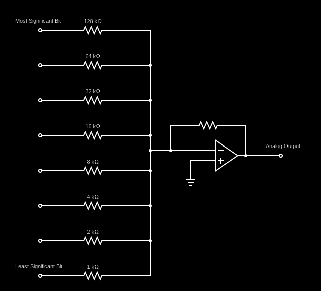
If you look at the resistances of the resistors attached to each of the bits of the binary input, you can see that they double from one input to another from the least significant bit to the most significant. This is extremely similar to what the network learned to do with the weights of the input layer. The main difference is that the weights are duplicated between each of the two 8-bit inputs. This allows the network to both sum the inputs as well as convert the sum to analog all within a single layer/neuron and do it all before any activation functions even come into play.
This was only part of the puzzle, though. Once the digital inputs were converted to analog and summed together, they were immediately passed through the neuron's activation function. To help track down what happened next, I plotted the post-activation outputs of a few of the neurons in the first layer as the inputs increased:
The neurons seemed to be generating sine wave-like outputs that changed smoothly as the sum of the binary inputs increased. Different neurons had different periods; the ones pictured above have periods of 8, 4, and 32 respectively. Other neurons had different periods or were offset by certain distances.
There's something very remarkable about this pattern: they map directly to the periods at which different binary digits switch between 0 and 1 when counting in binary. The least significant digit switches between 0 and 1 with a period of 1, the second with a period of 2, and so on to 4, 8, 16, 32, etc. This means that for at least some of the output bits, the network had learned to compute everything it needed in a single neuron.
Looking at the weights of neurons in the two later layers confirms this to be the case. The later layers are mostly concerned with routing around the outputs from the first layer and combining them. One additional benefit that those layers provide is "saturating" the signals and making them more square wave-like - pushing them closer to the target values of -1 and 1 for all values. This is the exact same property which is used in digital signal processing for audio synthesis where tanh is used to add distortion to sound for things like guitar pedals.
While playing around with this setup, I tried re-training the network with the activation function for the first layer replaced with sin(x) and it ends up working pretty much the same way. Interestingly, the weights learned in that case are fractions of π rather than 1.
For other output digits, the network learned to do some over clever things to generate the output signals it needed. For example, it combined outputs from the first layer in such a way that it was able to produce a shifted version of the signal not present in any of the first-layer neurons by adding signals from other neurons with different periods together. It worked out pretty well, more than accurate enough for the purpose of the network.
What it did ends up being roughly equivalent to the following sine-based version:

Again, I must say that I have no idea if this is just another random mathematical coincidence or part of some infinite series or something, but it's very neat regardless.
As I mentioned, before, I had imagined the network learning some fancy combination of logic gates to perform the whole addition process digitally, similarly to how a binary adder operates. This trick is yet another example of neural networks finding unexpected ways to solve problems. I was certainly amazed when I first figured out what it was doing and how it worked. I'm even more impressed that it manages to learn these features so consistently; all the first layer neurons end up taking on patterns similar to these every time I've trained it.
After all that, I'm not sure if this result can be used in support of or against the practical utility of the Ameo activation function. It definitely "worked" and solved it well, but it almost felt like cheating. In any case, I really enjoyed reverse engineering its solution and seeing all the ideas from digital signal processing and electronics it used to produce it.
Epilogue
This post certainly covered a lot of ground - from logic gates to activation functions to boolean complexity to electronics. When I started working on all of this, I didn't set out with the goal of going down the rabbit hole this far, but everything is so closely related to everything else in this space that it almost felt necessary in order to understand the bigger picture. Pulling one thread keeps bringing in a ton of other ideas and concepts.
Here's an example. All information flowing through ANNs takes the form of matrixes of numbers. The output of any layer in a network can be interpreted as a point in n-dimensional space. Using dimensionality reduction techniques like PCA or UMAP, that data information be compressed (lossily) and converted down into a lower dimensional space. Abstract concepts like computational complexity, information, probability, entropy, and logic can be expressed in terms of distances and space, thus allowing them to be understood visually and interacted with in a way that's familiar to the human brain.
The concept of embeddings, which I've written about in the past in the context of music, are based on this idea. Information, in the form of nodes in a graph, can be assigned coordinates in n-dimensional space in such a way that the information contained in the underlying graph is preserved. The famous example is the ability to operate on word embeddings using simple math in order to do things like king - man + woman = queen.
I feel like that's at the root of the lesson - if any - that I've taken away from this work. I believe that neural networks are as good as they are at what they do because of how low level and fundamental their components are. Other models of computation like Turing machines or finite state machines are elegant and perfect, but they feel much more mechanical and artificial. This is unsurprising given the biological inspiration for artificial neural networks and the mathematical origins of the others.
In any case, I've greatly enjoyed exploring these topics. For things that are often described as impenetrable "black boxes", I've found that neural networks actually have a lot to say about both how they model things and about information and computation in general.