Topic Modeling
Topic modeling is a natural language processing (NLP) technique for determining the topics in a document. Also, we can use it to discover patterns of words in a collection of documents. By analyzing the frequency of words and phrases in the documents, it’s able to determine the probability of a word or phrase belonging to a certain topic and cluster documents based on their similarity or closeness.
Firstly, topic modeling starts with a large corpus of text and reduces it to a much smaller number of topics. Topics are found by analyzing the relationship between words in the corpus. Also, topic modeling finds which words frequently co-occur with others and how often they appear together.
The model tries to find clusters of words that co-occur more frequently than they would otherwise expect due to chance alone. This gives a rough idea about topics in the document and where they rank on its hierarchy of importance.
The current methods for extraction of topic models include Latent Dirichlet Allocation (LDA), Latent Semantic Analysis (LSA), Probabilistic Latent Semantic Analysis (PLSA), and Non-Negative Matrix Factorization (NMF). In this article, we’ll focus on Latent Dirichlet Allocation (LDA).
The reason topic modeling is useful is that it allows the user to not only explore what’s inside their corpus (documents) but also build new connections between topics they weren’t even aware of. Some applications of topic modeling also include text summarization, recommender systems, spam filters, and similar.
Latent Dirichlet Allocation (LDA)
Latent Dirichlet Allocation (LDA) is an unsupervised clustering technique that is commonly used for text analysis. It’s a type of topic modeling in which words are represented as topics, and documents are represented as a collection of these word topics.
For this purpose, we’ll describe the LDA through topic modeling. Thus, let’s imagine that we have a collection of documents or articles. Each document has a topic such as computer science, physics, biology, etc. Also, some of the articles might have multiple topics. The problem is that we have only articles but not their topics and we would like to have an algorithm that is able to sort documents into topics.
Sampling Topics
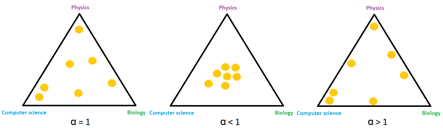
We can imagine that LDA will place documents in the space according to the document topics. For example, in our case with topics computer science, physics, and biology, LDA will put documents into a triangle where corners are the topics. We can see this in the image below where each orange circle represents one document.

As we’ve said, some documents might have several topics and an example of that is the document between computer science and biology in the image above. For instance, it’s possible if the document is about biotechnology. In probability and statistics, such kind of distribution is called Dirichlet distribution and it’s controlled by the parameter \(\alpha\).
For example, \(\alpha=1\) indicates that samples are more evenly distributed over the space, \(\alpha>1\) means that samples are gathering in the middle, and \(\alpha<1\) indicates that samples tend towards corners. Also, parameter \(\alpha\) is usually a \(k\)-dimensional vector, where each component corresponds to each corner or topic in our case. We can observe this behavior in the image below.
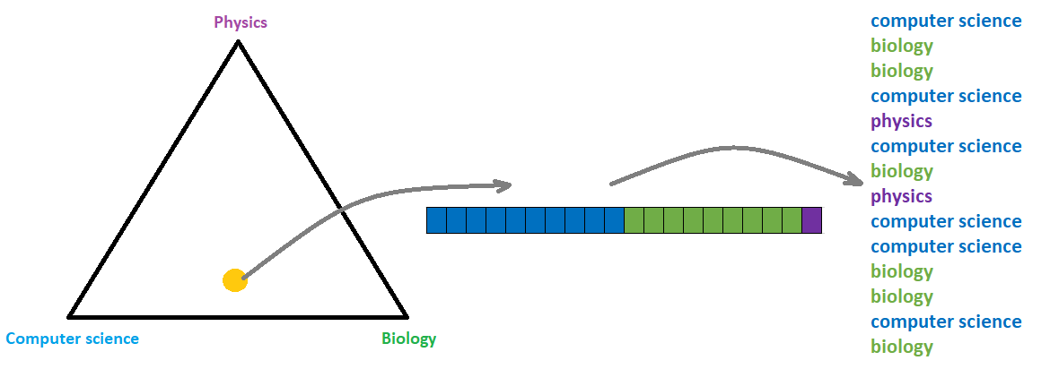
Next, if we consider the document about biotechnology that we mentioned above, it might consist of 50% computer science, 45% biology, and 5% physics. Generally, we can define this distribution of topics over a document as multinomial distribution with parameter \(\theta\). Accordingly, the \(\theta\) parameter is a \(k\)-dimensional vector of probabilities, which must sum to 1. After that, we sample from the multinomial distribution \(N\) different topics. In order to understand this process, we can observe the image below.
Sampling Words
After picking \(N\) different topics, we would also need to sample words. For that purpose, we’ll also use Dirichlet and multinomial distribution. The second Dirichlet distribution, defined with parameter \(\beta\), maps topics in word space. For instance, the corners of a triangle, tetrahedron in case of 4 dimensions or simplex for \(n\) dimensions, might be now words such as algorithm, genetic, velocity, or similar.
Instead of documents, now we are placing topics into this space. For example, the topic of computer science is closer to the word algorithm rather than to the word genetic, and the multinomial distribution of words for this topic might consist of 75% algorithm, 15% genetic, and 10% velocity. Similarly, we can define multinomial distributions for topic biology as 10% algorithm, 85% genetic, and 5% velocity, and topic physics as 20% algorithm, 5% genetic, and 75% velocity.
Also, after defining multinomial distributions for topics, we’ll sample words from those distributions corresponding to each topic sampled in the first step. This process can be more easily understood through the illustration below.
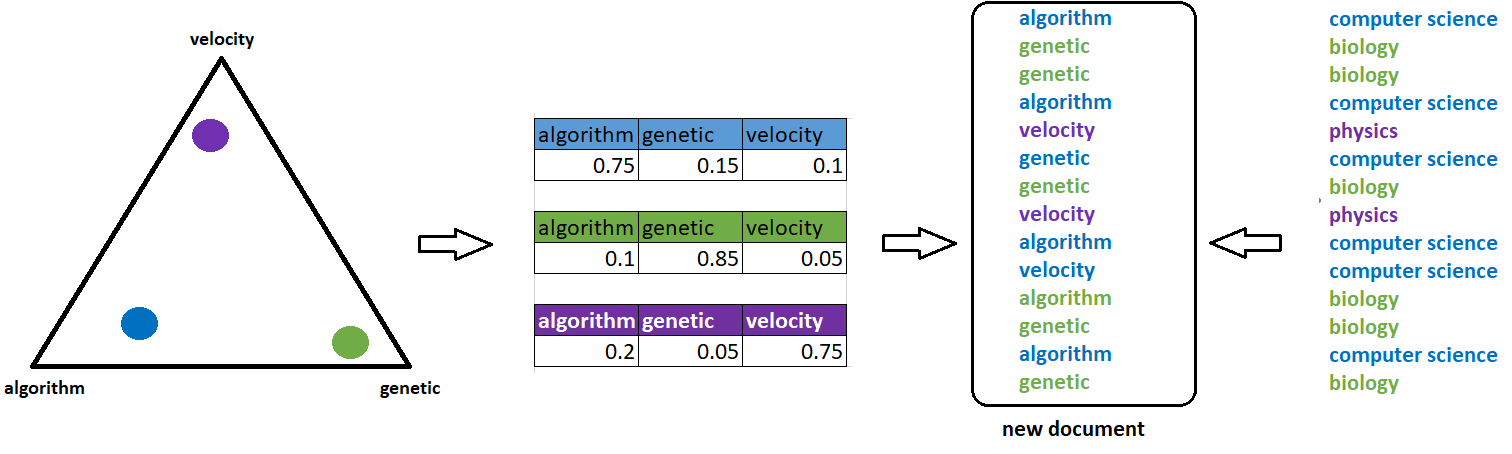
For example, if we consider a blue circle that represents a computer science topic, this topic has its own distribution by words that we’re using. Next, following the same order of sampled topics, for each topic, we select one word based on the topics distribution. For instance, the first topic above is computer science, and based on probability 0.75, 0.15, and 0.1 for words algorithm, genetic, and velocity respectively, we selected the word algorithm. Following this process, LDA creates a new document.
LDA Definition
In this way, for each input document, we create a new one. After all, we want to maximize the probability of creating the same document and the whole process above is mathematically defined as
$$
P(\boldsymbol{W}, \boldsymbol{Z}, \boldsymbol{\theta}, \boldsymbol{\phi}; \alpha, \beta) = \prod_{i = 1}^{M}P(\theta_{j}; \alpha)\prod_{i = 1}^{K}P(\phi; \beta)\prod_{t = 1}^{N}P(Z_{j, t} | \theta_{j})P(W_{j, t} | \phi z_{j, t}),
$$
\(\alpha\) and \(\beta\) define Dirichlet distributions, \(\theta\) and \(\phi\) define multinomial distributions, \(\boldsymbol{Z}\) is the vector with topics of all words in all documents, \(\boldsymbol{W}\) is the vector with all words in all documents, \(M\) number of documents, \(K\) number of topics and \(N\) number of words.
The whole process of training or maximizing probability can be done using Gibbs sampling where the general idea is to make each document and each word as monochromatic as possible. Basically, it means we want that each document have as few as possible articles and each word belongs to as few as possible topics.
Example
In this example, we’ll use the 20 newsgroups text dataset. The 20 newsgroups dataset comprises around 12000 newsgroups posts on 20 topics. Let’s load the data and all the needed packages.
import pandas as pd
import re
import numpy as np
from sklearn.datasets import fetch_20newsgroups
import nltk
from nltk.stem import WordNetLemmatizer
from nltk.corpus import stopwords

from gensim import corpora, models
from gensim.models.ldamulticore import LdaMulticore
from gensim.models.coherencemodel import CoherenceModel
import pyLDAvis.gensim
newsgroups_train = fetch_20newsgroups(subset='train')

df = pd.DataFrame({'post': newsgroups_train['data'], 'target': newsgroups_train['target']})
df['target_names'] = df['target'].apply(lambda t: newsgroups_train['target_names'][t])
df.head()
 	post 	target 	target_names
0 	From: [email protected] (where's my thing)\nS... 	7 	rec.autos
1 	From: [email protected] (Guy Kuo)... 	4 	comp.sys.mac.hardware
2 	From: [email protected] (Thomas E Will... 	4 	comp.sys.mac.hardware
3 	From: jgreen@amber (Joe Green)\nSubject: Re: W... 	1 	comp.graphics
4 	From: [email protected] (Jonathan McDow... 	14 	sci.space
As a text preprocessing step, we’ll first remove URLs, HTML tags, emails, and non-alpha characters. After that, we’ll lemmatize it and remove stopwords.
def remove_urls(text):
    " removes urls"
    url_pattern = re.compile(r'https?://\S+|www\.\S+')
    return url_pattern.sub(r'', text)

def remove_html(text):
    " removes html tags"
    html_pattern = re.compile('')
    return html_pattern.sub(r'', text)

def remove_emails(text):
    email_pattern = re.compile('\S*@\S*\s?')
    return email_pattern.sub(r'', text)

def remove_new_line(text):
    return re.sub('\s+', ' ', text)

def remove_non_alpha(text):
    return re.sub("[^A-Za-z]+", ' ', str(text))

def preprocess_text(text):
    t = remove_urls(text)
    t = remove_html(t)
    t = remove_emails(t)
    t = remove_new_line(t)
    t = remove_non_alpha(t)
    return t

def lemmatize_words(text, lemmatizer):
    return " ".join([lemmatizer.lemmatize(word) for word in text.split()])

def remove_stopwords(text, stopwords):
    return " ".join([word for word in str(text).split() if word not in stopwords])


df['post_preprocessed'] = df['post'].apply(preprocess_text).str.lower()

print('lemming...')
nltk.download('wordnet')
lemmatizer = WordNetLemmatizer()
df['post_final'] = df['post_preprocessed'].apply(lambda post: lemmatize_words(post, lemmatizer))

print('remove stopwors...')

nltk.download('stopwords')
swords = set(stopwords.words('english'))

df['post_final'] = df['post_preprocessed'].apply(lambda post: remove_stopwords(post, swords))
df.head()

	post 	target 	target_names 	post_preprocessed 	post_final
0 	From: [email protected] (where's my thing)\nS... 	7 	rec.autos 	from where s my thing subject what car is this... 	thing subject car nntp posting host rac wam um...
1 	From: [email protected] (Guy Kuo)... 	4 	comp.sys.mac.hardware 	from guy kuo subject si clock poll final call ... 	guy kuo subject si clock poll final call summa...
2 	From: [email protected] (Thomas E Will... 	4 	comp.sys.mac.hardware 	from thomas e willis subject pb questions orga... 	thomas e willis subject pb questions organizat...
3 	From: jgreen@amber (Joe Green)\nSubject: Re: W... 	1 	comp.graphics 	from joe green subject re weitek p organizatio... 	joe green subject weitek p organization harris...
4 	From: [email protected] (Jonathan McDow... 	14 	sci.space 	from jonathan mcdowell subject re shuttle laun... 	jonathan mcdowell subject shuttle launch quest...
Next, we’ll make the dictionary and corpus. Also, as a corpus, we can use only term frequency or TF-IDF.
posts = [x.split(' ') for x in df['post_final']]
id2word = corpora.Dictionary(posts)
corpus_tf = [id2word.doc2bow(text) for text in posts]
print(corpus_tf[0])
[(0, 1), (1, 2), (2, 1), (3, 1), (4, 1), (5, 1), (6, 1), (7, 5), (8, 1), (9, 1), (10, 1), (11, 1), (12, 1), (13, 1), (14, 1), (15, 1), (16, 1), (17, 1), (18, 1), (19, 1), (20, 1), (21, 1), (22, 1), (23, 1), (24, 1), (25, 1), (26, 1), (27, 1), (28, 1), (29, 1), (30, 1), (31, 1), (32, 1), (33, 1), (34, 1), (35, 1), (36, 1), (37, 1), (38, 1), (39, 1), (40, 1), (41, 1), (42, 1), (43, 1), (44, 1), (45, 1), (46, 1), (47, 1), (48, 1), (49, 1), (50, 1), (51, 1), (52, 1), (53, 1), (54, 1), (55, 1), (56, 1), (57, 1), (58, 1), (59, 1)]
tfidf = models.TfidfModel(corpus_tf)
corpus_tfidf = tfidf[corpus_tf]
print(corpus_tfidf[0])
[(0, 0.11498876048525103), (1, 0.09718324368673029), (2, 0.10251459464215813), (3, 0.22950467156922127), (4, 0.11224887707193924), (5, 0.1722981301822569), (6, 0.07530011969613486), (7, 0.4309484809469165), (8, 0.08877590143625969), (9, 0.04578068195160004), (10, 0.07090803901993002), (11, 0.1222656727768876), (12, 0.14524649469964415), (13, 0.05251249361530128), (14, 0.0989263305425191), (15, 0.04078267609390185), (16, 0.11756371552272524), (17, 0.17436169259993298), (18, 0.10155337594190954), (19, 0.20948825386578207), (20, 0.09695491629716278), (21, 0.024520714650907785), (22, 0.12964907508803875), (23, 0.08179595178219969), (24, 0.035633159058452026), (25, 0.11020678338364179), (26, 0.24952108927266048), (27, 9.459268363417395e-05), (28, 0.10776183582290975), (29, 0.07547376776331942), (30, 0.06670829980433708), (31, 0.062106577059591), (32, 0.13626396477950442), (33, 0.10453869332078215), (34, 0.07661054771383646), (35, 0.17037224424255862), (36, 0.024905114157890113), (37, 0.0011640619492058468), (38, 0.12139841280668175), (39, 0.054717960920777436), (40, 0.02308905209371841), (41, 0.13459748784234876), (42, 0.20608696405865523), (43, 0.056503689640334795), (44, 0.09456465243547033), (45, 0.09876981207502786), (46, 0.12006279504111743), (47, 0.08461773880033642), (48, 0.13486864088205006), (49, 0.13432885719305454), (51, 0.24952108927266048), (52, 0.05421309514981315), (53, 0.064793199454388), (54, 0.16160262905222716), (55, 0.027057268862720633), (56, 0.1954679598913907), (57, 0.09504085428857881), (58, 0.105116264304804), (59, 0.06248175923527969)]
After that, we test both corpus using the LDA model. We’ll measure their performance using coherence score UMass as a more commonly used CV score might not give good results. More about coherence scores can be found in this article.
In order to see keywords for each topic, we use method `show_topics`. Basically, it shows the topic index and weightage of each keyword.
model = LdaMulticore(corpus=corpus_tf,id2word = id2word, num_topics = 20,
                     alpha=.1, eta=0.1, random_state = 0)

coherence = CoherenceModel(model = model, texts = posts, dictionary = id2word, coherence = 'u_mass')

print(coherence.get_coherence())
print(model.show_topics())
-1.6040665431701946
[(6, '0.010*"god" + 0.008*"people" + 0.007*"one" + 0.006*"would" + 0.006*"subject" + 0.005*"lines" + 0.004*"article" + 0.004*"writes" + 0.004*"organization" + 0.004*"may"'),
 (12, '0.008*"subject" + 0.008*"lines" + 0.008*"organization" + 0.006*"article" + 0.006*"writes" + 0.006*"would" + 0.005*"one" + 0.005*"x" + 0.004*"university" + 0.004*"posting"'),
...
...
Visualize the topics-keywords
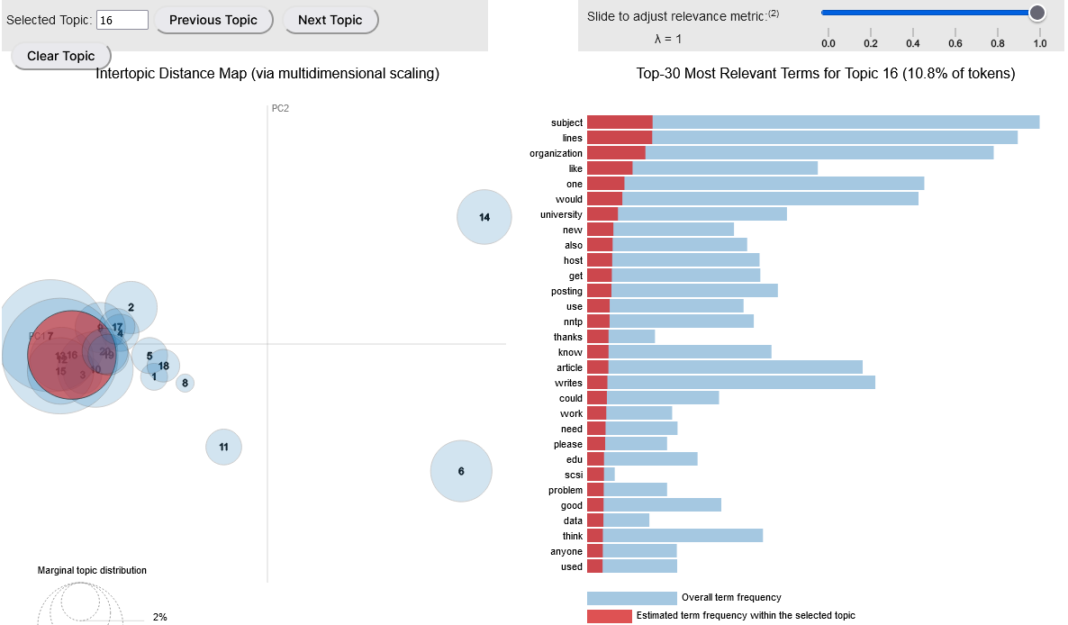
After we built the LDA model, the next step is to visualize results using pyLDAvis package. It’s an interactive chart that shows topics and keywords.
On the left side, topics are represented as circles. The larger the circle, the more prevalent is that topic. A good topic model will have big, non-overlapping circles scattered throughout the chart instead of being clustered in one quadrant.
On the right side, we can observe the most relevant keywords from the selected topic.
lda_display = pyLDAvis.gensim.prepare(model, corpus_tf, id2word, sort_topics = False)
pyLDAvis.display(lda_display)
In the end, dominant topic and contribution percent of that topic is extracted.
data_dict = {'dominant_topic':[], 'perc_contribution':[], 'topic_keywords':[]}

for i, row in enumerate(model[corpus_tf]):
    #print(i)
    row = sorted(row, key=lambda x: x[1], reverse=True)
    #print(row)
    for j, (topic_num, prop_topic) in enumerate(row):
        wp = model.show_topic(topic_num)
        topic_keywords = ", ".join([word for word, prop in wp])
        data_dict['dominant_topic'].append(int(topic_num))
        data_dict['perc_contribution'].append(round(prop_topic, 3))
        data_dict['topic_keywords'].append(topic_keywords)
        #print(topic_keywords)
        break

df_topics = pd.DataFrame(data_dict)

contents = pd.Series(posts)

df_topics['post'] = df['post']
df_topics.head()
Further work
This tutorial represents only the theoretical background and baseline model for topic modeling and the LDA algorithm. Thus, the presented results might not be the best possible, and a lot of space is left for improving them. For instance, we might try using different text preprocessing methods, tune LDA hyperparameters, such as the number of topics, alpha, beta, try different coherence metrics, and similar.
References
- Latent Dirichlet Allocation (Part 1 and 2), https://www.youtube.com/watch?v=T05t-SqKArY
- Topic Modeling With Gensim (Python), https://www.machinelearningplus.com/nlp/topic-modeling-gensim-python/
- When Coherence Score is Good or Bad in Topic Modeling?, https://www.baeldung.com/cs/topic-modeling-coherence-score
- Topic modeling guide (GSDM,LDA,LSI), https://www.kaggle.com/ptfrwrd/topic-modeling-guide-gsdm-lda-lsi
- Beginners Guide to Topic Modeling in Python, https://www.analyticsvidhya.com/blog/2016/08/beginners-guide-to-topic-modeling-in-python/