In my previous post, I showed how wonderful the ggplot2 library in R is for visualizing complex networks. I realized that while there are several posts on this blog going over the advanced visualization capabilities of the ggplot2 library, there isn’t a primer on structuring code for creating graphs in R…yet. In this post, I will go over the syntax for creating pretty ggplot2 graphs and tweaking various parameters. I am a self-declared Python aficionado, but love using ggplot2 because it is intuitive to use, beginner-friendly, and highly customizable all at the same time.

Dataset and setup

For this tutorial, I will be using one of the built-in datasets in R called mtcars which was extracted from the 1974 Motor Trend US magazine, and comprises fuel consumption and 10 aspects of automobile design and performance for 32 automobiles. Further documentation on this dataset can be found here. We import the data into our RStudio workspace.

# import the library into our workspace
library(ggplot2)

# import dataset
data(mtcars)
head(mtcars)

The resultant dataset looks something like this.

Basic plot

Now that we have the data, we can get to plotting with ggplot2. We can declaratively create graphics using this library. We just have to provide the data, specify how to map properties to graph aesthetics, and the library takes care of the rest for us! We need to specify three things for each ggplot — 1) the data, 2) the aesthetics, and 3) the geometry.

Let us start by creating a basic scatterplot of the mileage (mpg) of each car as a function of its horsepower (hp). In this case the data is our dataframe mtcars, and the aesthetics x and y will be defined as the names of the columns we wish to plot along each axis — hp and mpg. We can also set the color aesthetic to indicate the number of cylinders (cyl) in each car. One of the reasons ggplot2 is so user-friendly is because each graph property can be tacked on to the same line of code with a + sign. Since we want a scatterplot, the geometry will be defined using geom_point().

# basic scatterplot
g <- ggplot(data = mtcars, aes(x = hp, y = mpg, color=cyl))
g + geom_point()

Excellent! The library automatically assigns the column names as axis labels, and uses the default theme and colors, but all of this can be modified to suit our tastes and to create pretty graphs. It is also important to note that we could have visualized the same data (less helpfully) as a line plot instead of a scatterplot, just by tweaking the geometry function.

# basic line plot
g + geom_line()

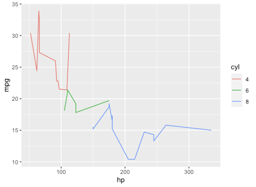
Well, this looks unpleasant. But wait, we can do so much more. We can also layer multiple geometries on the same graph to make more interesting plots.

# basic scatter+line plot
g + geom_line() + geom_point()

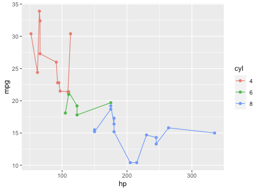
Additionally, we can tweak the geometry properties in each graph. Here is how we can transform the lines to dotted, and specify line widths and marker shape and size.

# change properties of geometry
g + geom_point(shape = "diamond", size = 3) +
  geom_line(color = "black", linetype = "dotted", size = .3) 

While our graph looks much neater now, using a line plot is actually pretty unhelpful for our dataset since each data point is a separate car. We will stick with a scatterplot for the rest of this tutorial. However, the above sort of graph would work great for time series data or other data that measures change in one variable.

Axis labels

One of the cardinal rules of good data visualization is to add axis labels to your graphs. While R automatically set the axis labels to be column headers, we can override this to make the axis labels more informative with just one extra function.

# change axis titles
g + geom_point(shape = "diamond", size = 3) +
  labs(x = "Horsepower (hp)", y = "Mileage (mpg)")

Title

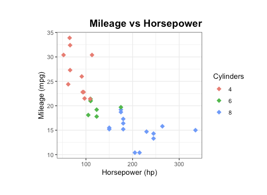
This graph is in serious need of a title to provide a reader some idea of what they’re looking at. There are actually multiple ways to add a graph title here, but I find it easiest to use ggtitle().

# add title
g + geom_point(shape = "diamond", size = 3) +
  labs(x = "Horsepower (hp)", y = "Mileage (mpg)") +
  ggtitle("Mileage vs Horsepower") 

Alright, having a title is helpful, but I don’t love it’s placement on the graph. R automatically left-aligns the title, where it clashes with the y-axis. I would much rather have the title right-aligned, in a bigger font, and bolded. Here is how to do that.

# change position of title
g + geom_point(shape = "diamond", size = 3) +
  labs(x = "Horsepower (hp)", y = "Mileage (mpg)") +
  ggtitle("Mileage vs Horsepower")  +
  theme(plot.title = element_text(hjust = 1, size = 15, face = "bold"))

Theme

There are ways to manually change the background and gridlines of ggplot2 graphs using theme(), but an easy workaround is to use the built-in themes. Which theme you use depends greatly on the graph type and formatting guidelines, but I personally like a white background, faint gridlines, and a bounding box. One thing to note here though is that theme_bw() overrides theme() so the order of these two matters.

# add theme
g + geom_point(shape = "diamond", size = 3) +
  labs(x = "Horsepower (hp)", y = "Mileage (mpg)") +
  ggtitle("Mileage vs Horsepower") +
  theme_bw() +
  theme(plot.title = element_text(hjust = 1, size = 15, face = "bold"))

We can also use the theme() function to change the base font size and font family. Shown below is how to increase the base font size to 15 and change the base font family to Courier.

# use theme to change base font family and font size
g + geom_point(shape = "diamond", size = 3) +
  labs(x = "Horsepower (hp)", y = "Mileage (mpg)") +
  ggtitle("Mileage vs Horsepower")  +
  theme_bw(base_size = 15, base_family = "Courier") +
  theme(plot.title = element_text(hjust = 1, size = 15, face = "bold"))

Legend

It has been bothering me for the last seven paragraphs that my legend title still uses the column name. However, this is an easy fix. All I have to do is add a label to the color aesthetic in the labs() function.

# change legend title
g + geom_point(shape = "diamond", size = 3) +
  labs(x = "Horsepower (hp)", y = "Mileage (mpg)", color = "Cylinders") +
  ggtitle("Mileage vs Horsepower") +
  theme_bw() +
  theme(plot.title = element_text(hjust = 1, size = 15, face = "bold"))

We can also change the position of the legend. R automatically places legends on the right, and while I like having it to the right in this case, I could also place the legend at the bottom of the graph. This automatically changes the aspect ratio of the graph.

# change legend position
g + geom_point(shape = "diamond", size = 3) +
  labs(x = "Horsepower (hp)", y = "Mileage (mpg)", color = "Cylinders") +
  ggtitle("Mileage vs Horsepower") +
  theme_bw() +
  theme(plot.title = element_text(hjust = 1, size = 15, face = "bold")) +
  theme(legend.position = "bottom")

Margins

The theme() function is of endless use in ggplot2, and can be used to manually adjust the graph margins and add/remove white space padding. The order of arguments in margin() is counterclockwise — top, right, bottom, left (helpfully remembered by the pneumonic TRouBLe).

# add plot margins
g + geom_point(shape = "diamond", size = 3) +
  labs(x = "Horsepower (hp)", y = "Mileage (mpg)", color = "Cylinders") +
  ggtitle("Mileage vs Horsepower") +
  theme_bw() +
  theme(plot.title = element_text(hjust = 1, size = 15, face = "bold")) +
  theme(legend.position = "right") +
  theme(plot.margin = margin(t = 1, r = 1, b = 1, l = 2, unit = "cm"))

Conclusion

I have barely scratched the surface of what can be achieved using ggplot2 in this post. There are hundreds of excellent tutorials online that dive deeper into ggplot2, like this blog post by Cedric Scherer. I have yet to learn so much about this library and data visualization in general, but have hopefully made a solid case for using ggplot2 to create clean and aesthetically-pleasing data visualizations.