A Gentle Introduction To Partial Derivatives and Gradient Vectors

Partial derivatives and gradient vectors are used very often in machine learning algorithms for finding the minimum or maximum of a function. Gradient vectors are used in the training of neural networks, logistic regression, and many other classification and regression problems.

In this tutorial, you will discover partial derivatives and the gradient vector.

After completing this tutorial, you will know:

• Function of several variables
• Level sets, contours and graphs of a function of two variables
• Partial derivatives of a function of several variables
• Gradient vector and its meaning

Let’s get started.

A Gentle Introduction To Partial Derivatives and Gradient Vectors. A photo by Atif Gulzar, some rights reserved.

Tutorial Overview

This tutorial is divided into three parts; they are:

1. Function of several variables
   1. Level sets
   2. Contours
   3. Graphs
2. Definition of partial derivatives
3. Gradient vector
   1. What does the gradient vector represent

A Function of Several Variables

You can review the concept of a function and a function of several variables in this tutorial.  We’ll provide more details about the functions of several variables here.

A function of several variables has the following properties:

• Its domain is a set of n-tuples given by (x_1, x_2, x_3, …, x_n)
• Its range is a set of real numbers

For example, the following is a function of two variables (n=2):

f_1(x,y) = x + y

In the above function x and y are the independent variables. Their sum determines the value of the function. The domain of this function is the set of all points on the XY cartesian plane. The plot of this function would require plotting in the 3D space, with two axes for input points (x,y) and the third representing the values of f.

Here is another example of a function of two variables. f_2(x,y) = x*x + y*y

To keep things simple, we’ll do examples of functions of two variables. Of course, in machine learning you’ll encounter functions of hundreds of variables. The concepts related to functions of two variables can be extended to those cases.

Level Sets and Graph of a Function of Two Variables

The set of points in a plane, where a function f(x,y) has a constant value, i.e., f(x,y)=c is the level set or level curve of f.

As an example, for function f_1, all (x,y) points that satisfy the equation below define a level set for f_1:

x + y = 1

We can see that this level set has an infinite set of points, e.g., (0,2), (1,1), (2, 0), etc. This level set defines a straight line in the XY plane.

In general, all level sets of f_1 define straight lines of the form (c is any real constant):

x + y = c

Similarly, for function f_2, an example of a level set is:

x*x + y*y = 1

We can see that any point that lies on a circle of radius 1 with center at (0,0) satisfies the above expression. Hence, this level set consists of all points that lie on this circle. Similarly, any level set of f_2 satisfies the following expression (c is any real constant >= 0):

x*x + y*y = c

Hence, all level sets of f_2 are circles with center at (0,0), each level set having its own radius.

The graph of the function f(x,y) is the set of all points (x,y,f(x,y)). It is also called a surface z=f(x,y). The graphs of f_1 and f_2 are shown below (left side).

The functions f_1 and f_2 and their corresponding contours

Contours of a Function of Two Variables

Suppose we have a function f(x,y) of two variables. If we cut the surface z=f(x,y) using a plane z=c, then we get the set of all points that satisfy f(x,y) = c. The contour curve is the set of points that satisfy f(x,y)=c, in the plane z=c. This is slightly different from the level set, where the level curve is directly defined in the XY plane. However, many books treat contours and level curves as the same.

The contours of both f_1 and f_2 are shown in the above figure (right side).

Partial Derivatives and Gradients

The partial derivative of a function f w.r.t. the variable x is denoted by ∂f/∂x. Its expression can be determined by differentiating f w.r.t. x. For example for the functions f_1 and f_2, we have:

∂f_1/∂x = 1

∂f_2/∂x = 2x

∂f_1/∂x represents the rate of change of f_1 w.r.t x. For any function f(x,y), ∂f/∂x represents the rate of change of f w.r.t variable x.

Similar is the case for ∂f/∂y. It represents the rate of change of f w.r.t y. You can look at the formal definition of partial derivatives in this tutorial.

When we find the partial derivatives w.r.t all independent variables, we end up with a vector. This vector is called the gradient vector of f denoted by ∇f(x,y). A general expression for the gradients of f_1 and f_2 are given by (here i,j are unit vectors parallel to the coordinate axis):

∇f_1(x,y) = ∂f_1/∂xi + ∂f_1/∂yj = i+j

∇f_2(x,y) = ∂f_2/∂xi + ∂f_2/∂yj = 2xi + 2yj

From the general expression of the gradient, we can evaluate the gradient at different points in space. In case of f_1 the gradient vector is a constant, i.e.,

i+j

No matter where we are in the three dimensional space, the direction and magnitude of the gradient vector remains unchanged.

For the function f_2, ∇f_2(x,y) changes with values of (x,y). For example, at (1,1) and (2,1) the gradient of f_2 is given by the following vectors:

∇f_2(1,1) = 2i + 2j

∇f_2(2,1) = 4i + 2j

What Does the Gradient Vector At a Point Indicate?

The gradient vector of a function of several variables at any point denotes the direction of maximum rate of change.

We can relate the gradient vector to the tangent line. If we are standing at a point in space and we come up with a rule that tells us to walk along the tangent to the contour at that point. It means wherever we are, we find the tangent line to the contour at that point and walk along it. If we walk following this rule, we’ll end up walking along the contour of f. The function’s value will never change as the function’s value is constant on the contour of f.

The gradient vector, on the other hand, is normal to the tangent line and points to the direction of maximum rate of increase. If we walk along the direction of the gradient we’ll start encountering the next point where the function’s value would be greater than the previous one.

The positive direction of the gradient indicates the direction of maximum rate of increase, whereas, the negative direction indicates the direction of maximum rate of decrease. The following figure shows the positive direction of the gradient vector at different points of the contours of function f_2. The direction of the positive gradient is indicated by the red arrow. The tangent line to a contour is shown in green.

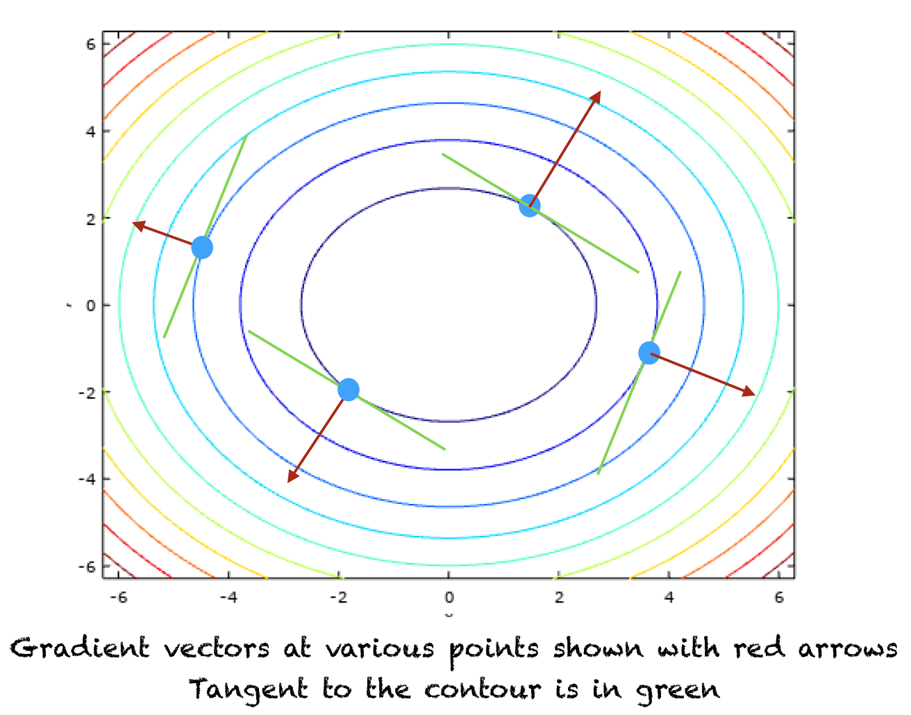
The contours and the direction of gradient vectors

Why Is The Gradient Vector Important In Machine Learning?

The gradient vector is very important and used frequently in machine learning algorithms. In classification and regression problems, we normally define the mean square error function. Following the negative direction of the gradient of this function will lead us to finding the point where this function has a minimum value.

Similar is the case for functions, where maximizing them leads to achieving maximum accuracy. In this case we’ll follow the direction of the maximum rate of increase of this function or the positive direction of the gradient vector.

Extensions

This section lists some ideas for extending the tutorial that you may wish to explore.

• Gradient descent/ gradient ascent
• Hessian matrix
• Jacobian

If you explore any of these extensions, I’d love to know. Post your findings in the comments below.

Further Reading

This section provides more resources on the topic if you are looking to go deeper.

Tutorials

• Derivatives
• Slopes and tangents
• Multivariate calculus
• Gradient descent for machine learning
• What is gradient in machine learning

Resources

• Additional resources on Calculus Books for Machine Learning

Books

• Thomas’ Calculus, 14th edition, 2017. (based on the original works of George B. Thomas, revised by Joel Hass, Christopher Heil, Maurice Weir)
• Calculus, 3rd Edition, 2017. (Gilbert Strang)
• Calculus, 8th edition, 2015. (James Stewart)

Summary

In this tutorial, you discovered what are functions of several variables, partial derivatives and the gradient vector. Specifically, you learned:

• Function of several variables
  • Contours of a function of several variables
  • Level sets of a function of several variables
• Partial derivatives of a function of several variables
• Gradient vector and its meaning

Do you have any questions?

Ask your questions in the comments below and I will do my best to answer.

Get a Handle on Calculus for Machine Learning!

Feel Smarter with Calculus Concepts

...by getting a better sense on the calculus symbols and terms

Discover how in my new Ebook:
Calculus for Machine Learning

It provides self-study tutorials with full working code on:
differntiation, gradient, Lagrangian mutiplier approach, Jacobian matrix, and much more...

Bring Just Enough Calculus Knowledge to
Your Machine Learning Projects

See What's Inside