This post is meant to be an introduction to convolutional neural networks (CNNs) and how they can be applied to continuous prediction problems, such as time series predictions. CNNs have historically been utilized in image classification applications. At a high level, CNNs use small kernels (filters) that can slide over localized regions of an image and detect features from edges to faces, much in the same way as the visual cortex of a brain (Hubel and Wiesel, 1968). The basic concepts of a CNN were first introduced by Kunihiko Fukushima in 1980 and the first use of CNNs for image recognition were carried out by Yann LeCun in 1988. The major breakthrough for the algorithm didn’t happen until 2000 with the advent of GPUs and by 2015, CNNs were favored to win image recognition contests over other deep networks.

It is believed that recurrent style networks such as LSTMs are the most appropriate algorithms for time series prediction, but studies have been conducted that suggest that CNNs can perform equivalently (or better) and that appropriate filters can extract features that are coupled across variables and time while being computationally efficient to train (Bai et al., 2018, Rodrigues et al., 2021). Below, I’ll demonstrate some of the key characteristics of CNNs and how CNNs can be used for time series prediction problems.

Architecture

Figure 1: CNN schematic for image classification (Sharma, 2018)

Figure 1 shows a schematic of a CNN’s architecture. The architecture is primarily comprised of a series of convolution and pooling layers followed by a fully connected network. In each convolution layer are kernel matrices that are convolved with the input into the convolution layer. It is up to the user to define the number of kernels and size of the kernels, but the weights in the kernel are learned using backpropagation. A bias is added to the output of the convolution layer and then passed through an activation function, such as ReLU function to yield feature maps. The feature maps are stacked in a cuboid of a depth that equals the number of filters. If the convolution layer is followed by a pooling layer, the feature maps are down-sampled to produce a lower dimensional representation of the feature maps. The output from the final pooling or convolutional layer is flattened and fed to the fully connected layers.

We will now look at the components of the architecture in more detail. To demonstrate how the convolutional layer works, we will use a toy example shown in Figure 2.

Figure 2: Convolution of a 3×3 kernel with the original image

Let’s say that our input is an image is represented as a 5×5 array and the filter is a 3×3 kernel that will be convolved with the image. The result is the array termed Conv1 which is just another array where each cell is the dot product between the filter and the 3×3 subsections of the image. The numbers in color represent the values that the filter is centered on. Note that the convolution operation will result in an output that is smaller than the input and can result in a loss of information around the boundaries of the image. Zero padding, which constitutes adding border of zeros around the input array, can be used to preserve the input size. The kernel matrices are the mechanisms by which the CNN is able to identify underlying patterns. Figure 3 shows examples of what successive output from convolution layers, or feature maps, can look like.

Figure 3: Convolutional layer output for a CNN trained to distinguish between cats and dogs (Dertat, 2017)

The filters in the first convolutional layer of a CNN retain most of the information of the image, particularly edges. The brightest colors represent the most active pixels. The feature maps tend to become more abstract or focused on specific features as you move deeper into the network (Dertat, 2017). For example, Block 3 seems to be tailored to distinguish eyes.

The other key type of layer is a pooling layer. A pooling layer is added after convolution to reduce dimensionality, which can both reduce computational time to train by reducing parameters but can also reduce the chances of overfitting. The most common type of pooling is max pooling which returns the max value in a NxN matrix pooling filter. This type of pooling retains the most active pixels in the feature map. As demonstrated in Figure 4, max pooling, using a 2×2 filter with a stride (or shift) of 2 pixels, reduces our Conv1 layer into a 2×2 lower dimensional matrix. One can also do average pooling instead of max pooling which would take the average of the values in each 2×2 subsection of the Conv1 layer.

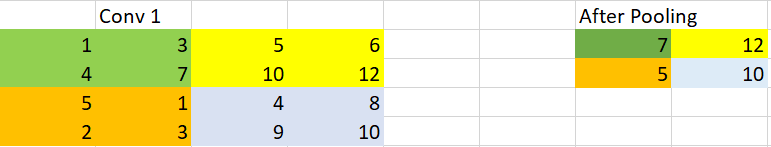
Figure 4: Max pooling example

Application to Regression

CNNs are easiest to understand and visualize for image applications which provide a basis for thinking about how we can use CNNs in a regression or prediction application for time series. Let’s use a very simple example of a rainfall-runoff problem that uses daily precipitation and temperature to predict outflow in an ephemeral sub-basin within the Tuolumne Basin. Because the sub-basin features a creek that is ephemeral, this means that the creek can dry up across the simulation period and there can be extended periods of zero flow. This can make predictions in the basin very difficult. Here, we also implement a lag which allows us to consider the residence time of the basin and that precipitation/temperature from days before likely will contribute to predicting the outflow today. We use a lag of 18, meaning that we use the previous 18 values of precipitation and temperature to predict outflow. The CNN model is implemented within Keras in the code below.

#import modules

import numpy as np
import pandas as pd
from keras.utils import to_categorical
from keras.models import Sequential, load_model
from keras.layers import LSTM, Dense
from keras.layers.convolutional import Conv1D, Conv2D
from keras.layers.convolutional import MaxPooling2D
from keras.layers import Dropout, Activation, Flatten
from keras.optimizers import SGD
import matplotlib.pyplot as plt
from sklearn.metrics import confusion_matrix
from sklearn.preprocessing import MinMaxScaler
from sklearn.model_selection import train_test_split
from tqdm import tqdm_notebook
import seaborn as sns
import os

os.getcwd()
os.chdir("C:/Users/Rohini/Documents/")
df_ge = pd.read_csv("Sub_0_daily.csv", index_col=0) 
print(df_ge.head())

#Check for nulls
print("checking if any null values are present\n", df_ge.isna().sum())

#Specify the training columns by their names
train_cols = ["Precipitation","Temperature"]
label_cols = ["Outflow"]



# This function normalizes the input data
def Normalization_Transform(x):
    x_mean=np.mean(x, axis=0)
    x_std= np.std(x, axis=0)
    xn = (x-x_mean)/x_std
    return xn, x_mean,x_std




# This function reverses the normalization 
def inverse_Normalization_Transform(xn, x_mean,x_std):
    xd = (xn*x_std)+x_mean
    return xd



# building timeseries data with given timesteps (lags)
def timeseries(X, Y, Y_actual, time_steps, out_steps):
    input_size_0 = X.shape[0] - time_steps
    input_size_1 = X.shape[1]
    X_values = np.zeros((input_size_0, time_steps, input_size_1))
    Y_values = np.zeros((input_size_0,))
    Y_values_actual = np.zeros((input_size_0,))
    
    for i in tqdm_notebook(range(input_size_0)):
        X_values[i] = X[i:time_steps+i]
        Y_values[i] = Y[time_steps+i-1, 0]
        Y_values_actual[i] = Y_actual[time_steps+i-1, 0]
        
    print("length of time-series i/o",X_values.shape,Y_values.shape)
    return X_values, Y_values, Y_values_actual


df_train, df_test = train_test_split(df_ge, train_size=0.8, test_size=0.2, shuffle=False)
x_train = df_train.loc[:,train_cols].values
y_train = df_train.loc[:,label_cols].values
x_test = df_test.loc[:,train_cols].values
y_test = df_test.loc[:,label_cols].values    
   
#Normalizing training data
x_train_nor = xtrain_min_max_scaler.fit_transform(x_train)
y_train_nor = ytrain_min_max_scaler.fit_transform(y_train)

# Normalizing test data
x_test_nor = xtest_min_max_scaler.fit_transform(x_test)
y_test_nor = ytest_min_max_scaler.fit_transform(y_test)

# Saving actual train and test y_label to calculate mean square error later after training
y_train_actual = y_train
y_test_actual = y_test

#Building timeseries
X_Train, Y_Train, Y_train_actual = timeseries(x_train_nor, y_train_nor, y_train_actual, time_steps=18, out_steps=1)
X_Test, Y_Test, Y_test_actual = timeseries(x_test_nor, y_test_nor, y_test_actual, time_steps=18, out_steps=1)

#Define CNN model

def make_model(X_Train):
    input_layer = Input(shape=(X_Train.shape[1],X_Train.shape[2]))

    conv1 = Conv1D(filters=16, kernel_size=2, strides=1,
                    padding='same',activation='relu')(input_layer)
    conv2 = Conv1D(filters=32, kernel_size=3,strides = 1,
                          padding='same', activation='relu')(conv1)
    conv3 = Conv1D(filters=64, kernel_size=3,strides = 1,
                          padding='same', activation='relu')(conv2)
    flatten = Flatten()(conv3)
    dense1 = Dense(1152, activation='relu')(flatten)
    dense2 = Dense(576, activation='relu')(dense1)
    output_layer = Dense(1, activation='linear')(dense2)
    
    return Model(inputs=input_layer, outputs=output_layer)

model = make_model(X_Train)
model.compile(optimizer = 'adam', loss = 'mean_squared_error')
model.fit(X_Train, Y_Train, epochs=10)


#Prediction and inverting results 
ypred = model.predict(X_Test)
predict =inverse_Normalization_Transform(ypred,y_mean_train, y_std_train)


#Plot results
plt.figure(figsize=(11, 7))

plt.plot(y_test)
plt.plot((predict))

plt.title('Outflow Prediction (Precipitation+Temperature,Epochs=10, Lag=18 hours)')
plt.ylabel('Outflow (cfs)')
plt.xlabel('Day')
plt.legend(['Actual Values','Predicted Values'], loc='upper right')
plt.show()

    

Just as with any algorithm, we normalize the input data and split it into testing and training sets. The CNN model is implemented in Keras and consists of three convolutional layers with kernel sizes that are explicitly defined to extract patterns that are coupled across variables and time. A schematic of the setup is shown in Figure 5.

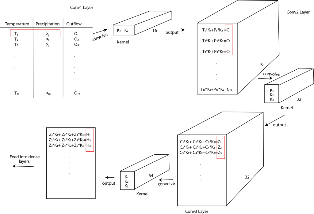
Figure 5: Convolution layer setup for the Tuolumne case

Layer 1 uses a 1D convolutional layer with 16 filters of size 1×2 in order to extract features and interactions across the precipitation and temperature time series as demonstrated in the top left of Figure 5. The result of this is an output layer of 1x18x16. The second convolution layer uses 32, 3×1 filters which now will further capture temporal interactions down the output column vector. The third layer uses 64, 3×1 filters to capture more complex temporal trends which is convolved with the output from the Conv2 layer. Note that zero padding is added (padding =”same” in the code) to maintain the dimensions of the layers. The three convolutional layers are followed by a flattening layer and a three-layer dense network. The CNN was run 20 times and the results from the last iteration are shown in Figure 6. We also compare to an LSTM that has an equivalent 3-layer setup and that is also run 20 times. The actual outflow is shown in blue while predictions are shown in red.

Figure 6: CNN vs LSTM prediction

For all purposes, the visual comparison yields that CNNs and LSTMs work equivalently, though the CNN was considerably faster to train. Notably, the CNN does a better job of capturing the large extremes recorded on day 100 and day 900, while still capturing the dynamics of the lower flow regime. While these results are preliminary and largely un-optimized, the CNN shows the ability to outperform an LSTM for a style of problem that it is not technically designed for. Using the specialized kernels, the CNN learns the interactions (both across variables and temporally) without needing a mechanism specifically designed for memory, such as a cell state in an LSTM. Furthermore, CNNs can greatly take advantage of additional speedups from GPUs which doesn’t always produce large gain in efficiency for LSTM training. For now, we can at least conclude that CNNs are fast and promising alternatives to LSTMs that you may not have considered before. Future blog posts will dive more into the capabilities of CNNs in problems with more input variables and complex interactions, particularly if there seems to be a benefit from CNNs in resolving complex relationships that help to predict extremes.

References

Hubel, D. H., & Wiesel, T. N. (1968). Receptive fields and functional architecture of monkey striate cortex. The Journal of physiology, 195(1), 215-243.

Bai, S., Kolter, J. Z., & Koltun, V. (2018). An empirical evaluation of generic convolutional and recurrent networks for sequence modeling. arXiv preprint arXiv:1803.01271.

Rodrigues, N. M., Batista, J. E., Trujillo, L., Duarte, B., Giacobini, M., Vanneschi, L., & Silva, S. (2021). Plotting time: On the usage of CNNs for time series classification. arXiv preprint arXiv:2102.04179.

Sharma, V. (2018). https://vinodsblog.com/2018/10/15/everything-you-need-to-know-about-convolutional-neural-networks/

Dertat, A. (2017). https://towardsdatascience.com/applied-deep-learning-part-4-convolutional-neural-networks-584bc134c1e2