Fitting discontinuous data from disparate sources
Sorting and searching are probably the most widely performed operations in computing; they are extensively covered in volume 3 of The Art of Computer Programming. Algorithm performance is influence by the characteristics of the processor on which it runs, and the size of the processor cache(s) has a significant impact on performance.
A study by Khuong and Morin investigated the performance of various search algorithms on 46 different processors. Khuong The two authors kindly sent me a copy of the raw data; the study webpage includes lots of plots.
The performance comparison involved 46 processors (mostly Intel x86 compatible cpus, plus a few ARM cpus) times 3 array datatypes times 81 array sizes times 28 search algorithms. First a 32/64/128-bit array of unsigned integers containing N elements was initialized with known values. The benchmark iterated 2-million times around randomly selecting one of the known values, and then searching for it using the algorithm under test. The time taken to iterate 2-million times was recorded. This was repeated for the 81 values of N, up to 63,095,734, on each of the 46 processors.
The plot below shows the results of running each algorithm benchmarked (colored lines) on an Intel Atom D2700 @ 2.13GHz, for 32-bit array elements; the kink in the lines occur roughly at the point where the size of the array exceeds the cache size (all code+data):
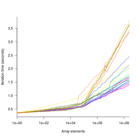
What is the most effective way of analyzing the measurements to produce consistent results?
One approach is to build two regression models, one for the measurements before the cache ‘kink’ and one for the measurements after this kink. By adding in a dummy variable at the kink-point, it is possible to merge these two models into one model. The problem with this approach is that the kink-point has to be chosen in advance. The plot shows that the performance kink occurs before the array size exceeds the cache size; other variables are using up some of the cache storage.
This approach requires fitting 46*3=138 models (I think the algorithm used can be integrated into the model).
If data from lots of processors is to be fitted, or the three datatypes handled, an automatic way of picking where the first regression model should end, and where the second regression model should start is needed.
Regression discontinuity design looks like it might be applicable; treating the point where the array size exceeds the cache size as the discontinuity. Traditionally discontinuity designs assume a sharp discontinuity, which is not the case for these benchmarks (R’s rdd package worked for one algorithm, one datatype running on one processor); the more recent continuity-based approach supports a transition interval before/after the discontinuity. The R package rdrobust supports a continued-based approach, but seems to expect the discontinuity to be a change of intercept, rather than a change of slope (or rather, I could not figure out how to get it to model a just change of slope; suggestions welcome).
Another approach is to use segmented regression, i.e., one of more distinct lines. The package segmented supports fitting this kind of model, and does estimate what they call the breakpoint (the user has to provide a first estimate).
I managed to fit a segmented model that included all the algorithms for 32-bit data, running on one processor (code+data). Looking at the fitted model I am not hopeful that adding data from more than one processor would produce something that contained useful information. I suspect that there are enough irregular behaviors in the benchmark runs to throw off fitting quality.
I’m always asking for more data, and now I have more data than I know how to analyze in a way that does not require me to build 100+ models 🙁
Suggestions welcome.
Came to your blog by the recent posts about code bureaucracy and research software. Looking at this post it seems I would have approached the curve fitting without seeing it as different models for different ranges, rather one curve model (function to map the abscissa-value to the ordinate-value) that is built up mathematically by an expression that includes enough parameters, e.g. including one for “turning point” (“cache size”). With the observation that a larger array is never going the make the running time shorter, we just need to add positive contributions.
I.e. something like:
t(N) = t0 + a*log10(N) + b*(log10(N)-log10(S))*(N>=S)
where (N>=S) means the Heaviside function of N-S or for a programmer simply means treating a boolean true as 1 and false as 0.
You would then run a nonlinear (least squares) regression with the parameters t0, a, b and S. If the startup time is negligible even for “small” arrays, we could drop the t0 completely. Since we can assume that the S-parameter relates to cache size, we could reduce the statistical uncertainty if we make a “global fit” of all results that used the same CPU and the same datatype (i.e. the cache size would correspond to the same number of array elements). However, if you want to test this hypothesis you must of course leave the the S-parameter free in the fitting and then test whether you found any significant deviation among the S fitted for the same (CPU, datatype)-tuple. A complication (or hypothesis to explore) here could be the whether the different algorithms consume a notably different amount of CPU-cache for instructions or other stuff, thereby giving different turning points S for the same CPU and datatype. With multiple levels of memory caches, the soft turning point you see could perhaps be a blurred result by a more complicated model having additional terms with a s1 and a s2 turning point?
If (since) you want to “smoothen” the single-turning-point model, a commonly occurring pattern can be something inspired by the 2-norm or sum of squares: rather than x + y we take sqrt(x^2 + y^2). When one of the terms is small, the result is approximately the absolute value of the dominant one, but there is never a sharp switchover point. We could try something like
t(N) = sqrt(t0^2 + (a*log10(N))^2 + (b*(log10(N)-log10(S))*(N>=S))^2)
or since the role of t0 will be confined to very small N and not so interesting I’d drop it and start with
t(N) = sqrt((a*log10(N))^2 + (b*(log10(N)-log10(S))*(N>=S))^2)
You link to a Wikipedia page about “regression discontinuity design” but as you pointed out your curve doesn’t look discontinuous, only the first derivative is discontinuous if we make a curve with a “sharp slope change” while keeping the curve “connected”. That would be my first equation, without any square-root. Visually and numerically I’d claim that the square-root of squared terms goes one step further by making also the first derivative continuous, but I haven’t bothered to differentiate it analytically to prove it.
Finally, it is not obvious to me what “consistent results” you need. What question/hypothesis do you want to answer/test? What aspect do you want to compare or optimize? I believe your signal to noise is good enoguh to fit this kind of model on individual curves as a “data reduction” stage, so that you only have the few parameters to then tabulate/visualize between the algorithms, CPUs and datatypes.
For a quick visualization in Python I did:
import numpy as np
from matplotlib import pyplot as plt
x = np.arange(0, 9, 0.01) # x could be your log10(N), so I let s=log10(S)
model_1 = lambda x, s, t0, a, b: t0 + a*x + b*(x-s)*(x>s)
model_2 = lambda x, s, t0, a, b: np.sqrt(t0**2+ (a*x)**2 + (b*(x-s)*(x>s))**2)
plt.plot(x, model_1(x, 4, 1, 1.5, 5), x, model_2(x, 4, 1, 2, 6))
An extension, if you want to be able to find that (test whether) for some curves there is no effect of cache-size, i.e. just a single slope all the way, you could enter the domain of “Model selection” with nested models.
Basically the reduced model t(N) = t0 + a*log10(N) is nested within the model t(N) = t0 + a*log10(N) + b*(log10(N)-log10(S))*(N>=S), because we can always achieve the reduced result by picking a specific value of the extra b-parameter (b=0, S doesn’t matter). Consequently, a fit with the full model is always following the data points at least as good as the reduced model does.
The question that model selection aims to answer is whether the improved fit by adding two parameters (b and S) is “worth it” or “significant” enough to justify the larger number of parameters.
There is a big comment on https://stats.stackexchange.com/questions/219319/what-statistical-test-to-use-comparing-models that gives the key pointers, e.g. you could the log-likelihood ratio or the Akaike information criterion for two slightly different but well-justified ways of making the decision. Both of them require calculating the likelihood of your fit (see below) and then use either the concept of “degrees of freedom” or “number of parameters” to penalize each model’s “score”.
https://en.wikipedia.org/wiki/Degrees_of_freedom_(statistics)#In_structural_equation_models
https://en.wikipedia.org/wiki/Akaike_information_criterion#Counting_parameters
To compute the likelihood function’s value (needed for both approaches) you need to decide what statistical distribution you assume for your data. I find the Wikipedia page https://en.wikipedia.org/wiki/Likelihood_function rather big and scary without any relevant example. Although there are some larger fluctuations in the curves when the time is long than when short, a first guess could be that the the time of each data point is normally distributed with the same standard deviation for all points. This would make the expression for the likelihood as on https://www.statlect.com/fundamentals-of-statistics/normal-distribution-maximum-likelihood
Using the Akaike (AIC) approach we want to express the difference AIC1 − AIC2 = 2*(k1−k2) +2*(ln(L2)−ln(L1)), and prefer model 2 if this is positive and model 1 if negative.
The equations for “log-likelihood function” from the last link is the same as the slightly less clearly expressed on https://en.wikipedia.org/wiki/Akaike_information_criterion#Comparison_with_least_squares
where they also conclude what applies when we make the assumption of identical normally distributed noise, i.e. the both the sigma-estimate and the third term are given by the residual sum of squares, so the expression can be simplified slightly. The constant term (+C) can be ignored since we just care about the ln(L2)−ln(L1) difference where the identical C’s will cancel out (note that ln(L2)−ln(L1) = ln(L2/L1) is also called the log-likelihood ratio). Finally the k-values give the penalties based on number of parameters (counting the noise standard deviation as a parameter), i.e. k1=3 and k2=5.
You should of test an implementation of the model selection by running it on one of the datasets where it is obvious by eye that the b & S parameters are meaningful, then on a dataset (or faked points) where you can’t see any slope change and expect the reduced model to be preferred.
@Erik
Thanks for the detailed suggestions.
The first model you suggest is how I might have done it a few years ago, and still might these days, if I had a single dataset. See section 11.2.9 of my Evidence-based software engineering book.
With measurements of so many processors, I would like to compare behaviors, and the ‘kink’ moves around between processors and algorithms. Hence, my interest in methods that did not require me to hard-code a change-point.
Using a consistent approach across all data would enable values to be compared, e.g., value of ‘kink’ point and ration of before/after slopes.
A quadratic is a better fit for values before the ‘kink’, at least on the few samples I tried it on. Some samples are somewhat wavy, does this mean something happened during the measurement process, or are the results reality? More measurements are needed.
If it was not clear from my wall of text, I didn’t want you to hand-code the location of the “kink” (the s or S parameter). It should be fitted but together with the other parameters (a & b) by running a nonlinear least squares fit. (The second post is about auto-detecting the degenerate situation that some dataset (some algorithm) might not show a kink at all, then probably giving you very unreliable/random results for the s-parameter which “shouldn’t really be there”.)
A simple linear regression would only allow the a & b to be fitted while s has to be decided (manually) beforehand, so this might be what you had in mind. (The a and b are simple coefficients before some non-fitted expressions that can be computed before running the fitting of a and b to match a dataset).
A nonlinear optimization method (nonlinear least squares fitting) however allows any kind of parameter to be fitted, and thus all three parameters (a, b and s) to be fitted simultaneously starting from an initial guess. (The s parameter shifts the b-contribution sideways rather than acting as a coefficient.) As for the “manual” need to code an initial guess for all parameters, I would hope this model and data look rather robust against bad guesses, so I expect it to work with some shared constant initial guess for all datasets or some simple heuristics based on the min and max values, e.g. s = somewhere in the middle of the logarithmic N-range, a and b some constant fraction of the max(time)/max(N).
That “kink” seems a little late to be cache size. Are you sure it is not paging cost?
@Erik
Sorry for the delayed reply.
A nonlinear fit requires some initial values, and even then the algorithm is not guaranteed to converge. Yes, I think it could be made to work for one set of data, but I suspect that an attempt to fit lots of cpus with a general function will fail for a non-trivial percentage. This is my experience from fitting a fair few non-linear models.
Now, of course, the regression discontinuity algorithms may turn out to be just as ‘unfriendly’ as the non-linear ones. I don’t have much experience with them and so cannot say. But they are at least designed to handle this case, and I would expect them to do better.