Dijkstra’s algorithm in Python (Find Shortest Path)

Dijkstra’s algorithm operates on the principle of finding the shortest distance value of a node by iteration until it reaches the actual shortest distance.

A key aspect of Dijkstra’s algorithm is that it uses a priority queue to select the vertex with the smallest tentative distance from the set of nodes not yet processed.

The current node is marked as visited, and all its neighboring nodes are examined for a more optimal path.

The Dijkstra’s algorithm in Python would look something like this in action:

# Sample Graph represented as a dictionary
graph = {
  'A': {'B': 1, 'C': 4},
  'B': {'A': 9, 'D': 2},
  'C': {'A': 4, 'D': 6, 'F': 3},
  'D': {'B': 1, 'C': 1, 'E': 8},
  'E': {'D': 3},
  'F': {'C': 2}
}

def dijkstra(graph, start_node):
    pass  # algorithm implementation comes later

The dijkstra function is the algorithm’s primary implementation, taking the graph and the starting node as arguments.

 

 

Understanding Graph Theory

Before we dive deeper into the Dijkstra’s algorithm, it’s crucial to understand the basic principles of graph theory.

A graph is a mathematical structure that models the relationships between different objects. In the context of our tutorial, these objects are nodes in a graph.

The connections between these nodes are called edges. The nature of these edges and nodes defines the types of graphs, such as directed, undirected, weighted, and unweighted.

For Dijkstra’s shortest path algorithm, we generally use weighted and directed graphs, but the algorithm also works well with unweighted and undirected graphs.

Python code to create a graph is simple. For instance:

# Sample Graph represented as a dictionary
graph = {
  'A': {'B': 1, 'C': 4},
  'B': {'A': 9, 'D': 2},
  'C': {'A': 4, 'D': 6, 'F': 3},
  'D': {'B': 1, 'C': 1, 'E': 8},
  'E': {'D': 3},
  'F': {'C': 2}
}

This is a basic representation of a graph where ‘A’, ‘B’, ‘C’, ‘D’, ‘E’, and ‘F’ are nodes in the graph and the numbers are the weights of the edges between the nodes.

 

Components of a Graph: Nodes & Edges

A graph is comprised of two key components: Nodes and Edges. Nodes, also known as vertices, are the fundamental units of which graphs are formed.

They can represent various real-world entities such as cities on a map or web pages on the internet.

Edges, on the other hand, are the lines that connect these nodes. They can be either directed (one-way) or undirected (two-way).

In weighted graphs, edges also carry a value called ‘weight‘, which usually signifies the distance or cost between the two nodes.

To represent these components in Python, we often use data structures like lists, dictionaries, or a combination of both. Let’s see a code example:

# Defining nodes and edges
nodes = ["A", "B", "C", "D", "E", "F"]
edges = [("A", "B", 1), ("A", "C", 4), ("B", "D", 2), ("C", "D", 6), ("C", "F", 3), ("D", "E", 8), ("E", "D", 3), ("F", "C", 2)]

# Converting to a graph representation
graph = {node: {} for node in nodes}
for edge in edges:
    graph[edge[0]][edge[1]] = edge[2]

print(graph)

Output:

{
  'A': {'B': 1, 'C': 4},
  'B': {'D': 2},
  'C': {'D': 6, 'F': 3},
  'D': {'E': 8},
  'E': {'D': 3},
  'F': {'C': 2}
}

This code first defines nodes and edges. Then it transforms this information into a dictionary-based graph representation.

In this dictionary, each key-value pair corresponds to a node and its adjacent vertices, respectively.

The adjacency list is represented as another dictionary where each key-value pair corresponds to a neighboring node and the weight of the edge connecting the node pair, respectively.

Step-by-Step Explanation of the Algorithm

Here’s an overview of how Dijkstra’s algorithm works:

1. Initialize a dictionary that will store the shortest distances from the source to all other vertices.
2. Create a priority queue to hold the vertex with the smallest distance.
3. Set the distance from the source to the source itself as 0.
4. For the current node, consider all its unvisited neighboring nodes and calculate their tentative distance through the current node.
5. Compare the newly calculated tentative distance to the current assigned value and assign the smaller one.
6. Move the current node to the visited set; we’re done considering it.
7. Continue this process until all the vertices are visited.

import heapq
def dijkstra(graph, source):
    distance = {node: float('infinity') for node in graph}
    distance[source] = 0
    queue = [(0, source)]
    while queue:
        current_distance, current_node = heapq.heappop(queue)

        if current_distance > distance[current_node]:
            continue

        for neighbor, weight in graph[current_node].items():
            distance_through_current_node = current_distance + weight

            if distance_through_current_node < distance[neighbor]:
                distance[neighbor] = distance_through_current_node
                heapq.heappush(queue, (distance[neighbor], neighbor))

    return distance
print(dijkstra(graph, 'A'))

Output:

{'A': 0, 'B': 1, 'C': 4, 'D': 3, 'E': 11, 'F': 7}

In this code, we initialize the distance from the source node to all other nodes as infinity, except for the source node itself, which is 0. Then we start iterating over the graph from the source node.

The while loop runs until we have nodes in the queue. In each iteration, we pick a node with the smallest weight path from the start and consider all its unvisited neighbors.

If the calculated distance through the current node is less than the previously known distance, we update the shortest distance for that neighbor.

Once all nodes have been visited, we return the shortest distance from the source to all other vertices. The output is a dictionary with each node in the graph and the shortest distance from the source node.

 

Handling Edge Cases and Potential Errors

While implementing Dijkstra’s algorithm, you should be aware of certain edge cases and potential errors. Let’s discuss a few and how to handle them:

1. Empty Graph: An empty graph, with no nodes or edges, would result in an error since there’s no path to find. We should check if the graph is empty before running the algorithm.
2. Invalid Source Node: If the source node is not present in the graph, the algorithm will fail. We need to check if the source node exists in the graph.
3. Disconnected Graph: If the graph has two or more disconnected components, Dijkstra’s algorithm will not be able to find a path between nodes located in different components. This is not exactly an error, but an inherent limitation of the algorithm. The algorithm will still execute without issues, but the result might not be what you expect.
4. Negative Edge Weights: Dijkstra’s algorithm doesn’t handle negative edge weights. If your graph contains negative weights, you may want to use Bellman-Ford or Johnson’s algorithm.

Let’s handle these cases:

def dijkstra(graph, source):
    # Check if the graph is empty
    if not graph:
        return "Error: Graph is empty"

    # Check if the source node is valid
    if source not in graph:
        return "Error: Invalid source node"

    distance = {node: float('infinity') for node in graph}
    distance[source] = 0
    queue = [(0, source)]

    while queue:
        current_distance, current_node = heapq.heappop(queue)
        if current_distance > distance[current_node]:
            continue

        for neighbor, weight in graph[current_node].items():
            # Check for negative edge weights
            if weight < 0:
                return "Error: Graph contains negative edge weights"

            distance_through_current_node = current_distance + weight
            if distance_through_current_node < distance[neighbor]:
                distance[neighbor] = distance_through_current_node
                heapq.heappush(queue, (distance[neighbor], neighbor))
    return distance
print(dijkstra(graph, 'A'))

The output and explanation will remain the same as the previous section, but now, the function is more robust and can handle some edge cases and errors.

 

Visualizing Dijkstra’s Algorithm

Visualizing an algorithm like Dijkstra’s can greatly help in understanding how it operates and iterates over the graph to find the shortest paths.

We can do this using the matplotlib and networkx libraries in Python.

import networkx as nx
import matplotlib.pyplot as plt
G = nx.DiGraph()  # Create a new directed graph G

# Add edges with weights (replicating our example graph)
G.add_edge('A', 'B', weight=1)
G.add_edge('A', 'C', weight=4)
G.add_edge('B', 'D', weight=2)
G.add_edge('C', 'D', weight=6)
G.add_edge('C', 'F', weight=3)
G.add_edge('D', 'E', weight=8)

# Specify the positions of each node
pos = {'A': (0, 0), 'B': (1, 1), 'C': (1, -1), 'D': (2, 0), 'E': (3, 0), 'F': (2, -1)}

# Create edge labels for the weights
labels = nx.get_edge_attributes(G, 'weight')

# Draw the nodes
nx.draw_networkx_nodes(G, pos, node_color='orange')

# Draw the edges
nx.draw_networkx_edges(G, pos)

# Draw the node labels
nx.draw_networkx_labels(G, pos)

# Draw the edge labels
nx.draw_networkx_edge_labels(G, pos, edge_labels=labels)

plt.show()  # Display the graph

Output:

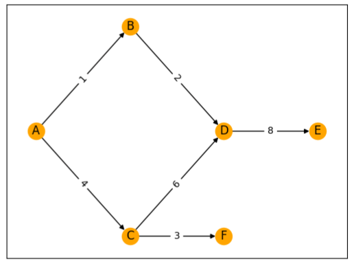
In this code, we use networkx to create a graph, add edges with weights, and specify the positions of each node. Then, we draw the nodes, edges, node labels, and edge labels (weights).

The final result is a visualized graph, which gives us a clear picture of how Dijkstra’s algorithm navigates through the graph to find the shortest paths.

 

Finding the Optimal Route from Two Starting Points

In some scenarios, you might want to determine the shortest path to a destination from two starting points.

The starting nodes will be start_node1 ‘A’ and start_node2 ‘B’ and the destination node is end_node ‘E’.

import heapq
def dijkstra(graph, start_node):
    distance = {node: float('inf') for node in graph}
    predecessor = {node: None for node in graph}
    distance[start_node] = 0
    queue = [(0, start_node)]
    while queue:
        current_distance, current_node = heapq.heappop(queue)

        for neighbor, weight in graph[current_node].items():
            new_distance = current_distance + weight
            if new_distance < distance[neighbor]:
                distance[neighbor] = new_distance
                predecessor[neighbor] = current_node
                heapq.heappush(queue, (new_distance, neighbor))
    return distance, predecessor

def find_shortest_path(graph, start_node1, start_node2, end_node):
    distance_from_start1, predecessor_from_start1 = dijkstra(graph, start_node1)
    distance_from_start2, predecessor_from_start2 = dijkstra(graph, start_node2)
    shortest_distance = min(
        distance_from_start1[end_node],
        distance_from_start2[end_node]
    )
    if shortest_distance == float('inf'):
        return None  # No path found
    path = [end_node]
    if distance_from_start1[end_node] <= distance_from_start2[end_node]:
        while path[-1] != start_node1:
            path.append(predecessor_from_start1[path[-1]])
    else:
        while path[-1] != start_node2:
            path.append(predecessor_from_start2[path[-1]])
    return path[::-1]
graph = {
    'A': {'B': 1, 'C': 4},
    'B': {'A': 9, 'D': 2},
    'C': {'A': 4, 'D': 6, 'F': 3},
    'D': {'B': 1, 'C': 1, 'E': 8},
    'E': {'D': 3},
    'F': {'C': 2}
}
start_node1 = 'A'
start_node2 = 'B'
end_node = 'E'

shortest_path = find_shortest_path(graph, start_node1, start_node2, end_node)
if shortest_path:
    print(f"Shortest path from either {start_node1} or {start_node2} to {end_node}: {' -> '.join(shortest_path)}")
else:
    print(f"No path found from either {start_node1} or {start_node2} to {end_node}")

Output:

Shortest path from either A or B to E: B -> D -> E

The function find_shortest_path(graph, start_node1, start_node2, end_node) calculates the shortest paths from both start_node1 and start_node2 to end_node.

It uses the above dijkstra function to get the distances and predecessor dictionaries for both start nodes.

The shortest distance to the end_node from either of the start nodes is then determined.

Using the appropriate predecessor dictionary, the function backtracks from the end node to the chosen starting node to construct the path.

We can visualize the graph using matplotlib for better understanding:

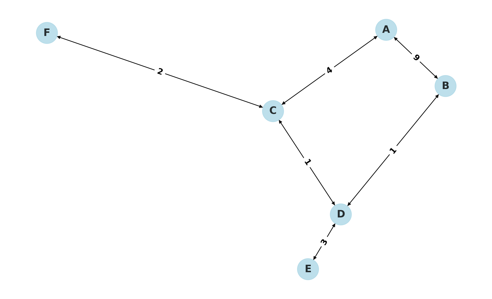
As you can see, the shortest path is B -> D -> E.

Highlight the shortest path

You can use networkx and matplotlib to visualize and highlight the path programmatically:

import networkx as nx
import matplotlib.pyplot as plt
def visualize_graph_with_highlighted_path(graph, shortest_path):
    G = nx.DiGraph()
    for node, neighbors in graph.items():
        for neighbor, weight in neighbors.items():
            G.add_edge(node, neighbor, weight=weight)

    pos = nx.spring_layout(G)
    nx.draw(G, pos, with_labels=True, node_size=800, node_color='lightgray', font_size=15)

    # If there's a shortest path, highlight it
    if shortest_path:
        path_edges = [(shortest_path[i], shortest_path[i+1]) for i in range(len(shortest_path)-1)]
        nx.draw_networkx_nodes(G, pos, nodelist=shortest_path, node_color='yellow', node_size=800)
        nx.draw_networkx_edges(G, pos, edgelist=path_edges, edge_color='blue', width=2.5, arrowstyle='-|>')
    plt.show()
visualize_graph_with_highlighted_path(graph, shortest_path)

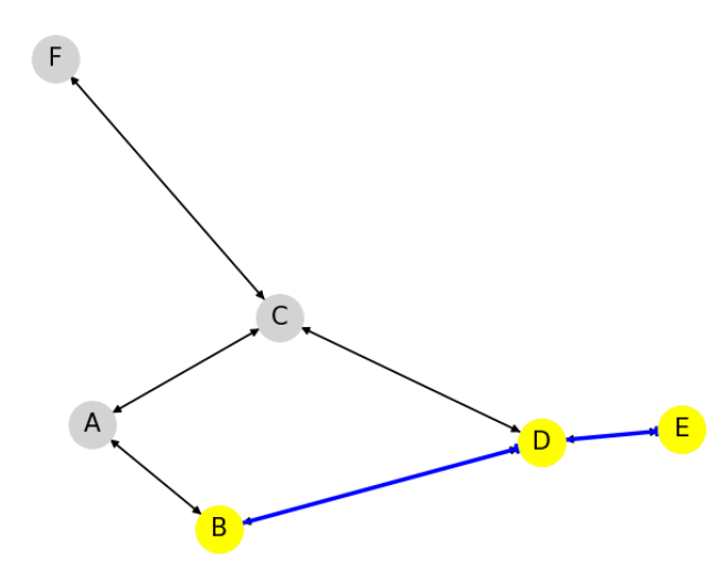
The nodes that are part of the shortest path are highlighted in yellow.

The edges forming the shortest path are shown in blue with wider lines and arrows.

 

Time Complexity Analysis

The time complexity of Dijkstra’s algorithm depends on the data structures used for the graph and for ordering the unvisited nodes according to their tentative distance from the source.

When using an adjacency matrix representation for the graph, the time complexity is O(V^2), where V is the number of vertices.

This is because we need to scan all nodes to pick the node with the minimum distance value. This approach is suitable when dealing with dense graphs, where the number of edges is close to V^2.

However, a more efficient approach for sparse graphs (where the number of edges is much less than V^2) is to use adjacency lists for the graph and a priority queue to extract nodes with the minimum distance. The most suitable data structure that can decrease the time complexity of Dijkstra’s algorithm to O((V+E)logV) is a binary heap.

In our Python implementation, we used the heapq module, which implements a binary heap, thus making the algorithm more efficient.

 

Space Complexity Analysis

The space complexity of Dijkstra’s algorithm in Python depends on the graph’s representation, specifically how we store the nodes and edges.

If we use an adjacency matrix to represent the graph, the space complexity will be O(V^2), where V is the number of vertices.

This is because we need to store all the edges for each node in the matrix, regardless of whether an edge between two nodes exists or not.

If we use an adjacency list, the space complexity will be O(V + E), where E is the number of edges. This is a more efficient method for sparse graphs where E is much less than V^2.

In the adjacency list representation, each node directly holds its neighbors, saving space.

In our Python implementation, we use a dictionary to implement the adjacency list, and we also keep a distance dictionary and a queue. Thus, the space complexity of our implementation is O(V + E).