
The Nelder-Mead optimization algorithm is a widely used approach for non-differentiable objective functions.
As such, it is generally referred to as a pattern search algorithm and is used as a local or global search procedure, challenging nonlinear and potentially noisy and multimodal function optimization problems.
In this tutorial, you will discover the Nelder-Mead optimization algorithm.
After completing this tutorial, you will know:
- The Nelder-Mead optimization algorithm is a type of pattern search that does not use function gradients.
- How to apply the Nelder-Mead algorithm for function optimization in Python.
- How to interpret the results of the Nelder-Mead algorithm on noisy and multimodal objective functions.
Kick-start your project with my new book Optimization for Machine Learning, including step-by-step tutorials and the Python source code files for all examples.
Let’s get started.
How to Use the Nelder-Mead Optimization in Python
Photo by Don Graham, some rights reserved.
Tutorial Overview
This tutorial is divided into three parts; they are:
- Nelder-Mead Algorithm
- Nelder-Mead Example in Python
- Nelder-Mead on Challenging Functions
- Noisy Optimization Problem
- Multimodal Optimization Problem
Nelder-Mead Algorithm
Nelder-Mead is an optimization algorithm named after the developers of the technique, John Nelder and Roger Mead.
The algorithm was described in their 1965 paper titled “A Simplex Method For Function Minimization” and has become a standard and widely used technique for function optimization.
It is appropriate for one-dimensional or multidimensional functions with numerical inputs.
Nelder-Mead is a pattern search optimization algorithm, which means it does not require or use function gradient information and is appropriate for optimization problems where the gradient of the function is unknown or cannot be reasonably computed.
It is often used for multidimensional nonlinear function optimization problems, although it can get stuck in local optima.
Practical performance of the Nelder–Mead algorithm is often reasonable, though stagnation has been observed to occur at nonoptimal points. Restarting can be used when stagnation is detected.
— Page 239, Numerical Optimization, 2006.
A starting point must be provided to the algorithm, which may be the endpoint of another global optimization algorithm or a random point drawn from the domain.
Given that the algorithm may get stuck, it may benefit from multiple restarts with different starting points.
The Nelder-Mead simplex method uses a simplex to traverse the space in search of a minimum.
— Page 105, Algorithms for Optimization, 2019.
The algorithm works by using a shape structure (called a simplex) composed of n + 1 points (vertices), where n is the number of input dimensions to the function.
For example, on a two-dimensional problem that may be plotted as a surface, the shape structure would be composed of three points represented as a triangle.
The Nelder-Mead method uses a series of rules that dictate how the simplex is updated based on evaluations of the objective function at its vertices.
— Page 106, Algorithms for Optimization, 2019.
The points of the shape structure are evaluated and simple rules are used to decide how to move the points of the shape based on their relative evaluation. This includes operations such as “reflection,” “expansion,” “contraction,” and “shrinkage” of the simplex shape on the surface of the objective function.
In a single iteration of the Nelder–Mead algorithm, we seek to remove the vertex with the worst function value and replace it with another point with a better value. The new point is obtained by reflecting, expanding, or contracting the simplex along the line joining the worst vertex with the centroid of the remaining vertices. If we cannot find a better point in this manner, we retain only the vertex with the best function value, and we shrink the simplex by moving all other vertices toward this value.
— Page 238, Numerical Optimization, 2006.
The search stops when the points converge on an optimum, when a minimum difference between evaluations is observed, or when a maximum number of function evaluations are performed.
Now that we have a high-level idea of how the algorithm works, let’s look at how we might use it in practice.
Want to Get Started With Optimization Algorithms?
Take my free 7-day email crash course now (with sample code).
Click to sign-up and also get a free PDF Ebook version of the course.
Nelder-Mead Example in Python
The Nelder-Mead optimization algorithm can be used in Python via the minimize() function.
This function requires that the “method” argument be set to “nelder-mead” to use the Nelder-Mead algorithm. It takes the objective function to be minimized and an initial point for the search.
|
1 2 3 |
... # perform the search result = minimize(objective, pt, method='nelder-mead') |
The result is an OptimizeResult object that contains information about the result of the optimization accessible via keys.
For example, the “success” boolean indicates whether the search was completed successfully or not, the “message” provides a human-readable message about the success or failure of the search, and the “nfev” key indicates the number of function evaluations that were performed.
Importantly, the “x” key specifies the input values that indicate the optima found by the search, if successful.
|
1 2 3 4 5 |
... # summarize the result print('Status : %s' % result['message']) print('Total Evaluations: %d' % result['nfev']) print('Solution: %s' % result['x']) |
We can demonstrate the Nelder-Mead optimization algorithm on a well-behaved function to show that it can quickly and efficiently find the optima without using any derivative information from the function.
In this case, we will use the x^2 function in two-dimensions, defined in the range -5.0 to 5.0 with the known optima at [0.0, 0.0].
We can define the objective() function below.
|
1 2 3 |
# objective function def objective(x): return x[0]**2.0 + x[1]**2.0 |
We will use a random point in the defined domain as a starting point for the search.
|
1 2 3 4 5 |
... # define range for input r_min, r_max = -5.0, 5.0 # define the starting point as a random sample from the domain pt = r_min + rand(2) * (r_max - r_min) |
The search can then be performed. We use the default maximum number of function evaluations set via the “maxiter” and set to N*200, where N is the number of input variables, which is two in this case, e.g. 400 evaluations.
|
1 2 3 |
... # perform the search result = minimize(objective, pt, method='nelder-mead') |
After the search is finished, we will report the total function evaluations used to find the optima and the success message of the search, which we expect to be positive in this case.
|
1 2 3 4 |
... # summarize the result print('Status : %s' % result['message']) print('Total Evaluations: %d' % result['nfev']) |
Finally, we will retrieve the input values for located optima, evaluate it using the objective function, and report both in a human-readable manner.
|
1 2 3 4 5 |
... # evaluate solution solution = result['x'] evaluation = objective(solution) print('Solution: f(%s) = %.5f' % (solution, evaluation)) |
Tying this together, the complete example of using the Nelder-Mead optimization algorithm on a simple convex objective function is listed below.
|
1 2 3 4 5 6 7 8 9 10 11 12 13 14 15 16 17 18 19 20 21 |
# nelder-mead optimization of a convex function from scipy.optimize import minimize from numpy.random import rand # objective function def objective(x): return x[0]**2.0 + x[1]**2.0 # define range for input r_min, r_max = -5.0, 5.0 # define the starting point as a random sample from the domain pt = r_min + rand(2) * (r_max - r_min) # perform the search result = minimize(objective, pt, method='nelder-mead') # summarize the result print('Status : %s' % result['message']) print('Total Evaluations: %d' % result['nfev']) # evaluate solution solution = result['x'] evaluation = objective(solution) print('Solution: f(%s) = %.5f' % (solution, evaluation)) |
Running the example executes the optimization, then reports the results.
Note: Your results may vary given the stochastic nature of the algorithm or evaluation procedure, or differences in numerical precision. Consider running the example a few times and compare the average outcome.
In this case, we can see that the search was successful, as we expected, and was completed after 88 function evaluations.
We can see that the optima was located with inputs very close to [0,0], which evaluates to the minimum objective value of 0.0.
|
1 2 3 |
Status: Optimization terminated successfully. Total Evaluations: 88 Solution: f([ 2.25680716e-05 -3.87021351e-05]) = 0.00000 |
Now that we have seen how to use the Nelder-Mead optimization algorithm successfully, let’s look at some examples where it does not perform so well.
Nelder-Mead on Challenging Functions
The Nelder-Mead optimization algorithm works well for a range of challenging nonlinear and non-differentiable objective functions.
Nevertheless, it can get stuck on multimodal optimization problems and noisy problems.
To make this concrete, let’s look at an example of each.
Noisy Optimization Problem
A noisy objective function is a function that gives different answers each time the same input is evaluated.
We can make an objective function artificially noisy by adding small Gaussian random numbers to the inputs prior to their evaluation.
For example, we can define a one-dimensional version of the x^2 function and use the randn() function to add small Gaussian random numbers to the input with a mean of 0.0 and a standard deviation of 0.3.
|
1 2 3 |
# objective function def objective(x): return (x + randn(len(x))*0.3)**2.0 |
The noise will make the function challenging to optimize for the algorithm and it will very likely not locate the optima at x=0.0.
The complete example of using Nelder-Mead to optimize the noisy objective function is listed below.
|
1 2 3 4 5 6 7 8 9 10 11 12 13 14 15 16 17 18 19 20 21 22 |
# nelder-mead optimization of noisy one-dimensional convex function from scipy.optimize import minimize from numpy.random import rand from numpy.random import randn # objective function def objective(x): return (x + randn(len(x))*0.3)**2.0 # define range for input r_min, r_max = -5.0, 5.0 # define the starting point as a random sample from the domain pt = r_min + rand(1) * (r_max - r_min) # perform the search result = minimize(objective, pt, method='nelder-mead') # summarize the result print('Status : %s' % result['message']) print('Total Evaluations: %d' % result['nfev']) # evaluate solution solution = result['x'] evaluation = objective(solution) print('Solution: f(%s) = %.5f' % (solution, evaluation)) |
Running the example executes the optimization, then reports the results.
Note: Your results may vary given the stochastic nature of the algorithm or evaluation procedure, or differences in numerical precision. Consider running the example a few times and compare the average outcome.
In this case, the algorithm does not converge and instead uses the maximum number of function evaluations, which is 200.
|
1 2 3 |
Status: Maximum number of function evaluations has been exceeded. Total Evaluations: 200 Solution: f([-0.6918238]) = 0.79431 |
The algorithm may converge on some runs of the code but will arrive on a point away from the optima.
Multimodal Optimization Problem
Many nonlinear objective functions may have multiple optima, referred to as multimodal problems.
The problem may be structured such that it has multiple global optima that have an equivalent function evaluation, or a single global optima and multiple local optima where algorithms like the Nelder-Mead can get stuck in search of the local optima.
The Ackley function is an example of the latter. It is a two-dimensional objective function that has a global optima at [0,0] but has many local optima.
The example below implements the Ackley and creates a three-dimensional plot showing the global optima and multiple local optima.
|
1 2 3 4 5 6 7 8 9 10 11 12 13 14 15 16 17 18 19 20 21 22 23 24 25 26 27 28 29 30 |
# ackley multimodal function from numpy import arange from numpy import exp from numpy import sqrt from numpy import cos from numpy import e from numpy import pi from numpy import meshgrid from matplotlib import pyplot from mpl_toolkits.mplot3d import Axes3D # objective function def objective(x, y): return -20.0 * exp(-0.2 * sqrt(0.5 * (x**2 + y**2))) - exp(0.5 * (cos(2 * pi * x) + cos(2 * pi * y))) + e + 20 # define range for input r_min, r_max = -5.0, 5.0 # sample input range uniformly at 0.1 increments xaxis = arange(r_min, r_max, 0.1) yaxis = arange(r_min, r_max, 0.1) # create a mesh from the axis x, y = meshgrid(xaxis, yaxis) # compute targets results = objective(x, y) # create a surface plot with the jet color scheme figure = pyplot.figure() axis = figure.gca(projection='3d') axis.plot_surface(x, y, results, cmap='jet') # show the plot pyplot.show() |
Running the example creates the surface plot of the Ackley function showing the vast number of local optima.
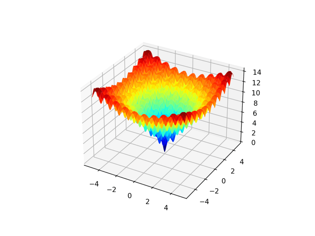
3D Surface Plot of the Ackley Multimodal Function
We would expect the Nelder-Mead function to get stuck in one of the local optima while in search of the global optima.
Initially, when the simplex is large, the algorithm may jump over many local optima, but as it contracts, it will get stuck.
We can explore this with the example below that demonstrates the Nelder-Mead algorithm on the Ackley function.
|
1 2 3 4 5 6 7 8 9 10 11 12 13 14 15 16 17 18 19 20 21 22 23 24 25 26 27 |
# nelder-mead for multimodal function optimization from scipy.optimize import minimize from numpy.random import rand from numpy import exp from numpy import sqrt from numpy import cos from numpy import e from numpy import pi # objective function def objective(v): x, y = v return -20.0 * exp(-0.2 * sqrt(0.5 * (x**2 + y**2))) - exp(0.5 * (cos(2 * pi * x) + cos(2 * pi * y))) + e + 20 # define range for input r_min, r_max = -5.0, 5.0 # define the starting point as a random sample from the domain pt = r_min + rand(2) * (r_max - r_min) # perform the search result = minimize(objective, pt, method='nelder-mead') # summarize the result print('Status : %s' % result['message']) print('Total Evaluations: %d' % result['nfev']) # evaluate solution solution = result['x'] evaluation = objective(solution) print('Solution: f(%s) = %.5f' % (solution, evaluation)) |
Running the example executes the optimization, then reports the results.
Note: Your results may vary given the stochastic nature of the algorithm or evaluation procedure, or differences in numerical precision. Consider running the example a few times and compare the average outcome.
In this case, we can see that the search completed successfully but did not locate the global optima. It got stuck and found a local optima.
Each time we run the example, we will find a different local optima given the different random starting point for the search.
|
1 2 3 |
Status: Optimization terminated successfully. Total Evaluations: 62 Solution: f([-4.9831427 -3.98656015]) = 11.90126 |
Further Reading
This section provides more resources on the topic if you are looking to go deeper.
Papers
Books
- Algorithms for Optimization, 2019.
- Numerical Optimization, 2006.
APIs
- Nelder-Mead Simplex algorithm (method=’Nelder-Mead’)
- scipy.optimize.minimize API.
- scipy.optimize.OptimizeResult API.
- numpy.random.randn API.
Articles
Summary
In this tutorial, you discovered the Nelder-Mead optimization algorithm.
Specifically, you learned:
- The Nelder-Mead optimization algorithm is a type of pattern search that does not use function gradients.
- How to apply the Nelder-Mead algorithm for function optimization in Python.
- How to interpret the results of the Nelder-Mead algorithm on noisy and multimodal objective functions.
Do you have any questions?
Ask your questions in the comments below and I will do my best to answer.
Get a Handle on Modern Optimization Algorithms!

Develop Your Understanding of Optimization
...with just a few lines of python code
Discover how in my new Ebook:
Optimization for Machine Learning
It provides self-study tutorials with full working code on:
Gradient Descent, Genetic Algorithms, Hill Climbing, Curve Fitting, RMSProp, Adam,
and much more...
")


Hi Jason,
Are you planning to write a practical optimisation book?
Matthew
I hope to.
I could not see why you are saying the Nelder Mead algorithm has an stochastic component. it is not an stochastic algorithm as for example the Simulation Annealing. Thus, if you start at the same point you should always get the same result.
Just the starting point for the search.
Used this method. As mentioned may get stuck at a local minima. Sometimes useful if the initial condition is the result of another optimization algorithm like Particle Swarm Optimization.
Could not agree more!!!
Jason, should the line be “… means it does *not* require or use function gradient….
“Nelder-Mead is a pattern search optimization algorithm, which means it does require or use function gradient information and is appropriate for optimization problems where the gradient of the function is unknown or cannot be reasonably computed.”
For sure, thanks, fixed.
Dear Dr Jason,
The Nelder-Mead optimization method can be used for non differentiable equations.
Examples of non-differential functions, y = |x|, y = x**0.5 and x**0.3333333, source, https://ocw.mit.edu/ans7870/18/18.013a/textbook/HTML/chapter06/section03.html.
This would imply that the Nelder-Mead optimzation may apply.
Question – when it comes to real-life data, how do know that the real-life data could belong to a non-differentiable function in order to apply the Nelder Mead optimization?
Thank you,
Anthony of Sydney
Yes, it can be used when you don’t have the derivative.
On a real project, you will know whether your objective is differentiable or not, and if you’re not sure you can try an auto-differentiation method to confirm.
Often we don’t have an equation, just a simulation (which is not differentiable).
Dear Dr Jason,
Thank you for the reply.
Question please: Where you say “…you will know whether your objective function is differentiable….” is that by looking at a plot of the graph of the real data and inspecting the graph, you look at the points of inflexion to see whether a tangent to the point of inflexion cannot be found?
Thank you again,
Anthony of Sydney
No, sorry. By that comment I meant you either have an equation or not. If you have an equation, you can either derive the derivative function or not.
Dear Dr Jason,
If you haven’t an equation but have real-life data and the data plotted on a graph and that graph looks like a function that looks undifferentiable.
Here is an example of y = |x| + noise
Suppose that this is real life data. How can we determine whether the real-life data follows a non differentiable function.
Thank you,
Anthony of Sydney
It is more complicated than that.
Consider the situation where you’re training a neural net on data.
The loss function is differentiable with regard to the model weights via the chain rule:
https://en.wikipedia.org/wiki/Chain_rule
For line 25 in the above code,
Replace
with
Thank you,
Anthony of Sydney
That was a good introduction to a whole world of optimism! I sometime feel that you read my google search and send me an email with the answer. I was researching this topic few days ago! Thanks again.
Thanks!
For those interested in the implementation details: The first time I saw an implementation of this algorithm (in Pascal) along with a good explanation was in Byte Magazine, May 1984, Volume 9 No 5, p.340:
“Fitting Curves to Data” by M.S. Cacechi and W.P. Cacheris.
Available in the Byte archive:
https://vintageapple.org/byte/pdf/198405_Byte_Magazine_Vol_09-05_Computers_and_the_Professions.pdf
https://archive.org/details/byte-magazine-1984-05/page/n347/mode/2up
I guess this reference places me firmly in the pre-Jurassic age 🙂
The Wikipedia article cited by Jason above has a nice animation.
Thanks for sharing!
Thanks for the info and sharing your knowledge
You’re welcome!
Thank you for a nice article.
One question: Do you know how to get confidence interval when using nelder mead in python?
Thank you.
Perhaps run with many different starting points and define an interval based on all final scores.
Hi, I am doing my university undergraduate project, and trying to convert MATLAB’s hybrid function to python. I plan to evaluate some of the benchmark functions such as rosenbrock, rastrigin,griewack,ackley,schewefel with a hybridized genetic algorithm which is GA+nelder-mead from scipy. Is it possible to do that in python? Like we did in matlab? Thanks
If so, I need to run the GA first, then runs the scipy after it terminates, or do I need to modify my GA?
Thanks alot, im very new to optimization.
I believe so.
This may help with the GA:
https://machinelearningmastery.com/simple-genetic-algorithm-from-scratch-in-python/
Thank you Jason for sharing this.
I am new to machine learning and currently working on a personal project. I am working on a regression problem using linear regression, tree based models(Decision tree and random forest) and an artificial neural network. I have got 11 numerical predictors.
I want to optimise all these models using this method but I have got a few questions.
1. Can this method be used for all the models listed above ?
2. How do I know the type of optimisation I am dealing with for each model i.e if it is convex, multimodal, noisy?
3. As I already have a trained model, I am guessing that would be my objective function.
4. How do I specify the r min, r max and pt?
(1) Nelder-Mead is to optimize a function. If you wrap your model as a function, you can apply this method.
(2) You never know if the model is too complex.
(3) If you already have a trained model, you have no objective function as there will be nothing for you to tune.
(4) You have to make these assumption.
One of the issues with Nelder-Mead is that of a large number of iterations frequently required. R defaults to 500 and for high dimension cases, that may not be enough. In many cases, the initial n+1 starting positions need to be randomly generated and it is therefore possible for such a polytope to be degenerate – a simple example is a triangle where 2 vertices are very close together. So::
1) Generate > n+1 (eg 2n) random locations.
2) Calculate the unit vectors between each pair of vertices.
3) Sort by their corresponding function results.
3) Start at the ‘best’ vertex, calculate the dot product of the unit vectors between each pair of the remaining vertices, the cosine of the angle.
4) If the dot product is above a critical value (eg 0.8), discard the poorer of the 2 vertices.
5) Terminate when there are n+1 ‘good’ locations.
Occasionally it is necessary generate another batch of vertices.
This is much simpler than trying to ensure that the polytope is convex, or estimating the hyper-volume to compare with a hyper-ball and I find that NM converges in 50-120 iterations in up to 40 dimensional problems.
Thank you for your feedback John! We appreciate it!
Hello, thank you for your example.
It needs an update:
MatplotlibDeprecationWarning: Calling gca() with keyword arguments was deprecated in Matplotlib 3.4. Starting two minor releases later, gca() will take no keyword arguments. The gca() function should only be used to get the current axes, or if no axes exist, create new axes with default keyword arguments. To create a new axes with non-default arguments, use plt.axes() or plt.subplot().
axis = figure.gca(projection=’3d’)
Without parameter:
axis.plot_surface(x, y, results, cmap=’jet’)
AttributeError: ‘AxesSubplot’ object has no attribute ‘plot_surface’
I am too unfamiliar with matplotlib…
Thank you for your feedback Sihir!