Multinomial Logistic Regression With Python

By Jason Brownlee on September 1, 2020 in Python Machine Learning 28

Multinomial logistic regression is an extension of logistic regression that adds native support for multi-class classification problems.

Logistic regression, by default, is limited to two-class classification problems. Some extensions like one-vs-rest can allow logistic regression to be used for multi-class classification problems, although they require that the classification problem first be transformed into multiple binary classification problems.

Instead, the multinomial logistic regression algorithm is an extension to the logistic regression model that involves changing the loss function to cross-entropy loss and predict probability distribution to a multinomial probability distribution to natively support multi-class classification problems.

In this tutorial, you will discover how to develop multinomial logistic regression models in Python.

After completing this tutorial, you will know:

Multinomial logistic regression is an extension of logistic regression for multi-class classification.
How to develop and evaluate multinomial logistic regression and develop a final model for making predictions on new data.
How to tune the penalty hyperparameter for the multinomial logistic regression model.

Let’s get started.

Multinomial Logistic Regression With Python
Photo by Nicolas Rénac, some rights reserved.

Tutorial Overview

This tutorial is divided into three parts; they are:

Multinomial Logistic Regression
Evaluate Multinomial Logistic Regression Model
Tune Penalty for Multinomial Logistic Regression

Multinomial Logistic Regression

Logistic regression is a classification algorithm.

It is intended for datasets that have numerical input variables and a categorical target variable that has two values or classes. Problems of this type are referred to as binary classification problems.

Logistic regression is designed for two-class problems, modeling the target using a binomial probability distribution function. The class labels are mapped to 1 for the positive class or outcome and 0 for the negative class or outcome. The fit model predicts the probability that an example belongs to class 1.

By default, logistic regression cannot be used for classification tasks that have more than two class labels, so-called multi-class classification.

Instead, it requires modification to support multi-class classification problems.

One popular approach for adapting logistic regression to multi-class classification problems is to split the multi-class classification problem into multiple binary classification problems and fit a standard logistic regression model on each subproblem. Techniques of this type include one-vs-rest and one-vs-one wrapper models.

An alternate approach involves changing the logistic regression model to support the prediction of multiple class labels directly. Specifically, to predict the probability that an input example belongs to each known class label.

The probability distribution that defines multi-class probabilities is called a multinomial probability distribution. A logistic regression model that is adapted to learn and predict a multinomial probability distribution is referred to as Multinomial Logistic Regression. Similarly, we might refer to default or standard logistic regression as Binomial Logistic Regression.

Binomial Logistic Regression: Standard logistic regression that predicts a binomial probability (i.e. for two classes) for each input example.
Multinomial Logistic Regression: Modified version of logistic regression that predicts a multinomial probability (i.e. more than two classes) for each input example.

If you are new to binomial and multinomial probability distributions, you may want to read the tutorial:

Discrete Probability Distributions for Machine Learning

Changing logistic regression from binomial to multinomial probability requires a change to the loss function used to train the model (e.g. log loss to cross-entropy loss), and a change to the output from a single probability value to one probability for each class label.

Now that we are familiar with multinomial logistic regression, let’s look at how we might develop and evaluate multinomial logistic regression models in Python.

Evaluate Multinomial Logistic Regression Model

In this section, we will develop and evaluate a multinomial logistic regression model using the scikit-learn Python machine learning library.

First, we will define a synthetic multi-class classification dataset to use as the basis of the investigation. This is a generic dataset that you can easily replace with your own loaded dataset later.

The make_classification() function can be used to generate a dataset with a given number of rows, columns, and classes. In this case, we will generate a dataset with 1,000 rows, 10 input variables or columns, and 3 classes.

The example below generates the dataset and summarizes the shape of the arrays and the distribution of examples across the three classes.

# test classification dataset
from collections import Counter
from sklearn.datasets import make_classification
# define dataset
X, y = make_classification(n_samples=1000, n_features=10, n_informative=5, n_redundant=5, n_classes=3, random_state=1)
# summarize the dataset
print(X.shape, y.shape)
print(Counter(y))

# test classification dataset

from collections import Counter

from sklearn.datasets import make_classification

# define dataset

X, y = make_classification(n_samples=1000, n_features=10, n_informative=5, n_redundant=5, n_classes=3, random_state=1)

# summarize the dataset

print(X.shape, y.shape)

print(Counter(y))

Running the example confirms that the dataset has 1,000 rows and 10 columns, as we expected, and that the rows are distributed approximately evenly across the three classes, with about 334 examples in each class.

(1000, 10) (1000,)
Counter({1: 334, 2: 334, 0: 332})

1 2	(1000, 10) (1000,) Counter({1: 334, 2: 334, 0: 332})

Logistic regression is supported in the scikit-learn library via the LogisticRegression class.

The LogisticRegression class can be configured for multinomial logistic regression by setting the “multi_class” argument to “multinomial” and the “solver” argument to a solver that supports multinomial logistic regression, such as “lbfgs“.

...
# define the multinomial logistic regression model
model = LogisticRegression(multi_class='multinomial', solver='lbfgs')

...

# define the multinomial logistic regression model

model = LogisticRegression(multi_class='multinomial', solver='lbfgs')

The multinomial logistic regression model will be fit using cross-entropy loss and will predict the integer value for each integer encoded class label.

Now that we are familiar with the multinomial logistic regression API, we can look at how we might evaluate a multinomial logistic regression model on our synthetic multi-class classification dataset.

It is a good practice to evaluate classification models using repeated stratified k-fold cross-validation. The stratification ensures that each cross-validation fold has approximately the same distribution of examples in each class as the whole training dataset.

We will use three repeats with 10 folds, which is a good default, and evaluate model performance using classification accuracy given that the classes are balanced.

The complete example of evaluating multinomial logistic regression for multi-class classification is listed below.

# evaluate multinomial logistic regression model
from numpy import mean
from numpy import std
from sklearn.datasets import make_classification
from sklearn.model_selection import cross_val_score
from sklearn.model_selection import RepeatedStratifiedKFold
from sklearn.linear_model import LogisticRegression
# define dataset
X, y = make_classification(n_samples=1000, n_features=10, n_informative=5, n_redundant=5, n_classes=3, random_state=1)
# define the multinomial logistic regression model
model = LogisticRegression(multi_class='multinomial', solver='lbfgs')
# define the model evaluation procedure
cv = RepeatedStratifiedKFold(n_splits=10, n_repeats=3, random_state=1)
# evaluate the model and collect the scores
n_scores = cross_val_score(model, X, y, scoring='accuracy', cv=cv, n_jobs=-1)
# report the model performance
print('Mean Accuracy: %.3f (%.3f)' % (mean(n_scores), std(n_scores)))

# evaluate multinomial logistic regression model

from numpy import mean

from numpy import std

from sklearn.datasets import make_classification

from sklearn.model_selection import cross_val_score

from sklearn.model_selection import RepeatedStratifiedKFold

from sklearn.linear_model import LogisticRegression

# define dataset

X, y = make_classification(n_samples=1000, n_features=10, n_informative=5, n_redundant=5, n_classes=3, random_state=1)

# define the multinomial logistic regression model

model = LogisticRegression(multi_class='multinomial', solver='lbfgs')

# define the model evaluation procedure

cv = RepeatedStratifiedKFold(n_splits=10, n_repeats=3, random_state=1)

# evaluate the model and collect the scores

n_scores = cross_val_score(model, X, y, scoring='accuracy', cv=cv, n_jobs=-1)

# report the model performance

print('Mean Accuracy: %.3f (%.3f)' % (mean(n_scores), std(n_scores)))

Running the example reports the mean classification accuracy across all folds and repeats of the evaluation procedure.

Note: Your results may vary given the stochastic nature of the algorithm or evaluation procedure, or differences in numerical precision. Consider running the example a few times and compare the average outcome.

In this case, we can see that the multinomial logistic regression model with default penalty achieved a mean classification accuracy of about 68.1 percent on our synthetic classification dataset.

Mean Accuracy: 0.681 (0.042)

1	Mean Accuracy: 0.681 (0.042)

We may decide to use the multinomial logistic regression model as our final model and make predictions on new data.

This can be achieved by first fitting the model on all available data, then calling the predict() function to make a prediction for new data.

The example below demonstrates how to make a prediction for new data using the multinomial logistic regression model.

# make a prediction with a multinomial logistic regression model
from sklearn.datasets import make_classification
from sklearn.linear_model import LogisticRegression
# define dataset
X, y = make_classification(n_samples=1000, n_features=10, n_informative=5, n_redundant=5, n_classes=3, random_state=1)
# define the multinomial logistic regression model
model = LogisticRegression(multi_class='multinomial', solver='lbfgs')
# fit the model on the whole dataset
model.fit(X, y)
# define a single row of input data
row = [1.89149379, -0.39847585, 1.63856893, 0.01647165, 1.51892395, -3.52651223, 1.80998823, 0.58810926, -0.02542177, -0.52835426]
# predict the class label
yhat = model.predict([row])
# summarize the predicted class
print('Predicted Class: %d' % yhat[0])

# make a prediction with a multinomial logistic regression model

from sklearn.datasets import make_classification

from sklearn.linear_model import LogisticRegression

# define dataset

X, y = make_classification(n_samples=1000, n_features=10, n_informative=5, n_redundant=5, n_classes=3, random_state=1)

# define the multinomial logistic regression model

model = LogisticRegression(multi_class='multinomial', solver='lbfgs')

# fit the model on the whole dataset

model.fit(X, y)

# define a single row of input data

row = [1.89149379, -0.39847585, 1.63856893, 0.01647165, 1.51892395, -3.52651223, 1.80998823, 0.58810926, -0.02542177, -0.52835426]

# predict the class label

yhat = model.predict([row])

# summarize the predicted class

print('Predicted Class: %d' % yhat[0])

Running the example first fits the model on all available data, then defines a row of data, which is provided to the model in order to make a prediction.

In this case, we can see that the model predicted the class “1” for the single row of data.

Predicted Class: 1

1	Predicted Class: 1

A benefit of multinomial logistic regression is that it can predict calibrated probabilities across all known class labels in the dataset.

This can be achieved by calling the predict_proba() function on the model.

The example below demonstrates how to predict a multinomial probability distribution for a new example using the multinomial logistic regression model.

# predict probabilities with a multinomial logistic regression model
from sklearn.datasets import make_classification
from sklearn.linear_model import LogisticRegression
# define dataset
X, y = make_classification(n_samples=1000, n_features=10, n_informative=5, n_redundant=5, n_classes=3, random_state=1)
# define the multinomial logistic regression model
model = LogisticRegression(multi_class='multinomial', solver='lbfgs')
# fit the model on the whole dataset
model.fit(X, y)
# define a single row of input data
row = [1.89149379, -0.39847585, 1.63856893, 0.01647165, 1.51892395, -3.52651223, 1.80998823, 0.58810926, -0.02542177, -0.52835426]
# predict a multinomial probability distribution
yhat = model.predict_proba([row])
# summarize the predicted probabilities
print('Predicted Probabilities: %s' % yhat[0])

# predict probabilities with a multinomial logistic regression model

from sklearn.datasets import make_classification

from sklearn.linear_model import LogisticRegression

# define dataset

X, y = make_classification(n_samples=1000, n_features=10, n_informative=5, n_redundant=5, n_classes=3, random_state=1)

# define the multinomial logistic regression model

model = LogisticRegression(multi_class='multinomial', solver='lbfgs')

# fit the model on the whole dataset

model.fit(X, y)

# define a single row of input data

row = [1.89149379, -0.39847585, 1.63856893, 0.01647165, 1.51892395, -3.52651223, 1.80998823, 0.58810926, -0.02542177, -0.52835426]

# predict a multinomial probability distribution

yhat = model.predict_proba([row])

# summarize the predicted probabilities

print('Predicted Probabilities: %s' % yhat[0])

Running the example first fits the model on all available data, then defines a row of data, which is provided to the model in order to predict class probabilities.

In this case, we can see that class 1 (e.g. the array index is mapped to the class integer value) has the largest predicted probability with about 0.50.

Predicted Probabilities: [0.16470456 0.50297138 0.33232406]

1	Predicted Probabilities: [0.16470456 0.50297138 0.33232406]

Now that we are familiar with evaluating and using multinomial logistic regression models, let’s explore how we might tune the model hyperparameters.

Tune Penalty for Multinomial Logistic Regression

An important hyperparameter to tune for multinomial logistic regression is the penalty term.

This term imposes pressure on the model to seek smaller model weights. This is achieved by adding a weighted sum of the model coefficients to the loss function, encouraging the model to reduce the size of the weights along with the error while fitting the model.

A popular type of penalty is the L2 penalty that adds the (weighted) sum of the squared coefficients to the loss function. A weighting of the coefficients can be used that reduces the strength of the penalty from full penalty to a very slight penalty.

By default, the LogisticRegression class uses the L2 penalty with a weighting of coefficients set to 1.0. The type of penalty can be set via the “penalty” argument with values of “l1“, “l2“, “elasticnet” (e.g. both), although not all solvers support all penalty types. The weighting of the coefficients in the penalty can be set via the “C” argument.

...
# define the multinomial logistic regression model with a default penalty
LogisticRegression(multi_class='multinomial', solver='lbfgs', penalty='l2', C=1.0)

...

# define the multinomial logistic regression model with a default penalty

LogisticRegression(multi_class='multinomial', solver='lbfgs', penalty='l2', C=1.0)

The weighting for the penalty is actually the inverse weighting, perhaps penalty = 1 – C.

From the documentation:

C : float, default=1.0
Inverse of regularization strength; must be a positive float. Like in support vector machines, smaller values specify stronger regularization.

This means that values close to 1.0 indicate very little penalty and values close to zero indicate a strong penalty. A C value of 1.0 may indicate no penalty at all.

C close to 1.0: Light penalty.
C close to 0.0: Strong penalty.

The penalty can be disabled by setting the “penalty” argument to the string “none“.

...
# define the multinomial logistic regression model without a penalty
LogisticRegression(multi_class='multinomial', solver='lbfgs', penalty='none')

...

# define the multinomial logistic regression model without a penalty

LogisticRegression(multi_class='multinomial', solver='lbfgs', penalty='none')

Now that we are familiar with the penalty, let’s look at how we might explore the effect of different penalty values on the performance of the multinomial logistic regression model.

It is common to test penalty values on a log scale in order to quickly discover the scale of penalty that works well for a model. Once found, further tuning at that scale may be beneficial.

We will explore the L2 penalty with weighting values in the range from 0.0001 to 1.0 on a log scale, in addition to no penalty or 0.0.

The complete example of evaluating L2 penalty values for multinomial logistic regression is listed below.

# tune regularization for multinomial logistic regression
from numpy import mean
from numpy import std
from sklearn.datasets import make_classification
from sklearn.model_selection import cross_val_score
from sklearn.model_selection import RepeatedStratifiedKFold
from sklearn.linear_model import LogisticRegression
from matplotlib import pyplot

# get the dataset
def get_dataset():
	X, y = make_classification(n_samples=1000, n_features=20, n_informative=15, n_redundant=5, random_state=1, n_classes=3)
	return X, y

# get a list of models to evaluate
def get_models():
	models = dict()
	for p in [0.0, 0.0001, 0.001, 0.01, 0.1, 1.0]:
		# create name for model
		key = '%.4f' % p
		# turn off penalty in some cases
		if p == 0.0:
			# no penalty in this case
			models[key] = LogisticRegression(multi_class='multinomial', solver='lbfgs', penalty='none')
		else:
			models[key] = LogisticRegression(multi_class='multinomial', solver='lbfgs', penalty='l2', C=p)
	return models

# evaluate a give model using cross-validation
def evaluate_model(model, X, y):
	# define the evaluation procedure
	cv = RepeatedStratifiedKFold(n_splits=10, n_repeats=3, random_state=1)
	# evaluate the model
	scores = cross_val_score(model, X, y, scoring='accuracy', cv=cv, n_jobs=-1)
	return scores

# define dataset
X, y = get_dataset()
# get the models to evaluate
models = get_models()
# evaluate the models and store results
results, names = list(), list()
for name, model in models.items():
	# evaluate the model and collect the scores
	scores = evaluate_model(model, X, y)
	# store the results
	results.append(scores)
	names.append(name)
	# summarize progress along the way
	print('>%s %.3f (%.3f)' % (name, mean(scores), std(scores)))
# plot model performance for comparison
pyplot.boxplot(results, labels=names, showmeans=True)
pyplot.show()

# tune regularization for multinomial logistic regression

from numpy import mean

from numpy import std

from sklearn.datasets import make_classification

from sklearn.model_selection import cross_val_score

from sklearn.model_selection import RepeatedStratifiedKFold

from sklearn.linear_model import LogisticRegression

from matplotlib import pyplot

# get the dataset

def get_dataset():

X, y = make_classification(n_samples=1000, n_features=20, n_informative=15, n_redundant=5, random_state=1, n_classes=3)

return X, y

# get a list of models to evaluate

def get_models():

models = dict()

for p in [0.0, 0.0001, 0.001, 0.01, 0.1, 1.0]:

# create name for model

key = '%.4f' % p

# turn off penalty in some cases

if p == 0.0:

# no penalty in this case

models[key] = LogisticRegression(multi_class='multinomial', solver='lbfgs', penalty='none')

else:

models[key] = LogisticRegression(multi_class='multinomial', solver='lbfgs', penalty='l2', C=p)

return models

# evaluate a give model using cross-validation

def evaluate_model(model, X, y):

# define the evaluation procedure

cv = RepeatedStratifiedKFold(n_splits=10, n_repeats=3, random_state=1)

# evaluate the model

scores = cross_val_score(model, X, y, scoring='accuracy', cv=cv, n_jobs=-1)

return scores

# define dataset

X, y = get_dataset()

# get the models to evaluate

models = get_models()

# evaluate the models and store results

results, names = list(), list()

for name, model in models.items():

# evaluate the model and collect the scores

scores = evaluate_model(model, X, y)

# store the results

results.append(scores)

names.append(name)

# summarize progress along the way

print('>%s %.3f (%.3f)' % (name, mean(scores), std(scores)))

# plot model performance for comparison

pyplot.boxplot(results, labels=names, showmeans=True)

pyplot.show()

Running the example reports the mean classification accuracy for each configuration along the way.

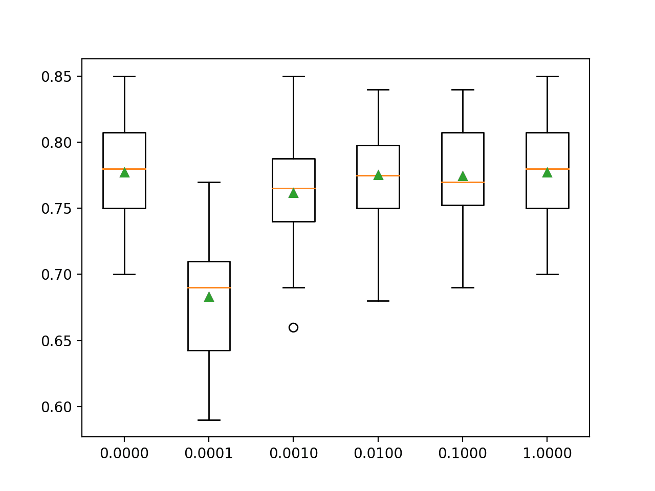
In this case, we can see that a C value of 1.0 has the best score of about 77.7 percent, which is the same as using no penalty that achieves the same score.

>0.0000 0.777 (0.037)
>0.0001 0.683 (0.049)
>0.0010 0.762 (0.044)
>0.0100 0.775 (0.040)
>0.1000 0.774 (0.038)
>1.0000 0.777 (0.037)

>0.0000 0.777 (0.037)

>0.0001 0.683 (0.049)

>0.0010 0.762 (0.044)

>0.0100 0.775 (0.040)

>0.1000 0.774 (0.038)

>1.0000 0.777 (0.037)

A box and whisker plot is created for the accuracy scores for each configuration and all plots are shown side by side on a figure on the same scale for direct comparison.

In this case, we can see that the larger penalty we use on this dataset (i.e. the smaller the C value), the worse the performance of the model.

Box and Whisker Plots of L2 Penalty Configuration vs. Accuracy for Multinomial Logistic Regression

Summary

In this tutorial, you discovered how to develop multinomial logistic regression models in Python.

Specifically, you learned:

Multinomial logistic regression is an extension of logistic regression for multi-class classification.
How to develop and evaluate multinomial logistic regression and develop a final model for making predictions on new data.
How to tune the penalty hyperparameter for the multinomial logistic regression model.

Do you have any questions?
Ask your questions in the comments below and I will do my best to answer.

28 Responses to Multinomial Logistic Regression With Python

Marry January 2, 2021 at 11:39 am #

Hi Jason,
Thank you so much for your informative and very educational blog. I am learning a lot from your site.
I am working with a machine learning project having ordinal target variable.
1- Do I consider it as a classification or regression problem?
2- If regression, which regression algorithm?
3- If classification, can I use Multinomial Logistic Regression for ordinal target?

Reply
- Jason Brownlee January 2, 2021 at 12:06 pm #
  
  You’re welcome.
  
  You can try modeling as classification and regression and see what works best.
  
  Try a suite of algorithms and discover what works best.
  
  Reply
Marry January 2, 2021 at 12:18 pm #

Thank you for your prompt response. Sorry, I am beginner in ML;I am a bit confused about the regression part. Does it mean I can try any of the regression algorithms regardless of the non-continuous nature of the target variable, which is ordinal (1-10)?

Reply
- Jason Brownlee January 3, 2021 at 5:51 am #
  
  Yes, although you may want to “interpret” the predictions, e.g. round to integer and calculate a metric that is meaningful to your project.
  
  Reply
sukhpal January 2, 2021 at 11:05 pm #

sir how we can further improve the decision making capabilities of the already optimized model

Reply
- Jason Brownlee January 3, 2021 at 5:55 am #
  
  Combine the prediction with other models, called an ensemble.
  
  Reply
marco January 2, 2021 at 11:52 pm #

Hello Jason,
do every scikit-learn and Xgbost estimators need that datasets have to be normalized/ standardized?
i.e. does it exist any estimator that allow input data as is?
Thanks,
Marco

Reply
- Jason Brownlee January 3, 2021 at 5:56 am #
  
  No.
  
  Trees can operate on raw data.
  
  Reply
marco January 2, 2021 at 11:53 pm #

Jason,
what are estimators suitable for unbalanced dataset?
Is the random forest suitable for predictions in healtcare where often dataset are unbalanced?
Thanks,
Marco

Reply
- Jason Brownlee January 3, 2021 at 5:57 am #
  
  Most can be used directly, some can be modified into cost-sensitive versions.
  
  Start here:
  https://machinelearningmastery.com/start-here/#imbalanced
  
  Reply
Albert March 14, 2021 at 1:48 am #

Hello Jason,

Thank you for the informative material.

I have been working with datasets having multiple classes such as the example above but I have found it difficult to plot RoC curves and calculate precision, recall, etc without using the OneVsRest method.

Can I work with just the multinomial class and then plot the RoC curve and calculate the rest?

Thanks in advance

Albert

Reply
- Jason Brownlee March 14, 2021 at 5:28 am #
  
  Perhaps this will help as a first step:
  https://machinelearningmastery.com/roc-curves-and-precision-recall-curves-for-classification-in-python/
  
  Reply
- Simon March 19, 2021 at 3:54 am #
  
  I wonder if you get any good answer on this? I’m in the same situation, I’m struggling to understand what the threshold should be for the multinormal case in terms of ROC curve.
  
  Reply
Oladiran Olanrewaju May 10, 2021 at 5:01 am #

Incase I want to generate multinomial data using Python. Please explain the steps

Reply
- Jason Brownlee May 10, 2021 at 6:22 am #
  
  Perhaps you can use make_classification():
  https://scikit-learn.org/stable/modules/generated/sklearn.datasets.make_classification.html
  
  Reply
Rusty November 3, 2021 at 4:21 am #

Hi Jason,

Thanks for such an instructive blog on machine learning.
I have one question: when you use RepeatedStratifiedKFold to evaluate the model and get the score out of it, but for predicting new data, out of these bunches of models (if n_splits=10, n_repeats=3, it will be 30 models, right?), which model should be selected to apply?

Thanks again!

Reply
- Adrian Tam November 7, 2021 at 7:23 am #
  
  For a correct use, none of these models should be selected. K-fold is to help you evaluate the model design. Once you finish with it, you should re-train the model with your full training set. See https://machinelearningmastery.com/training-validation-test-split-and-cross-validation-done-right/
  
  Reply
Luke May 25, 2022 at 1:55 pm #

Thank you for this article, I do have a question on the multinomial logistic regression. If I was interested on getting win probabilities for each horse in a horse race, if each row in the dataset had the prior average speed of each horse participating in the race, how would it be able to distinguish that say horse_1_speed in the first race (first row) is different than horse_1_speed in the second race (second row) since technically I can put any of the horses participating in that race as horse_1

Reply
- James Carmichael May 26, 2022 at 1:58 am #
  
  Hi Luke…Please narrow your query or rephrase in terms of a machine learning concept so that we may better assist you.
  
  Reply
Carol June 11, 2022 at 3:14 am #

When I use the Multinomial Logistic Regression I use the sigmoid function yet? Because if I have 2 classes I can calculate with sigmoid function. And with 3 classes or more, how I use this function?

Reply
- James Carmichael June 11, 2022 at 9:20 am #
  
  Hi Carol…The following may be of interest to you:
  
  https://towardsdatascience.com/multivariate-logistic-regression-in-python-7c6255a286ec
  
  Reply
skan January 11, 2023 at 6:41 am #

If I want to fit several logistic models… Do I need to instantiate them every time?
mymodel1 = LogisticRegression()
mymodel1.fit()
mymodel2 = LogisticRegression()
mymodel2.fit()
…

Reply
Gabriel February 25, 2023 at 9:01 am #

How do I know the type of distribution of my data? I have a database with categorical values, and all the attributes (input and output) has many categories. Could you tell me what algorithm is an approach to classify new values?

Reply
- James Carmichael February 25, 2023 at 10:13 am #
  
  Hi Gabriel…The following resource may be of interest to you:
  
  https://machinelearningmastery.com/statistical-data-distributions/
  
  Reply
Devon March 21, 2023 at 4:47 am #

Hi thanks for this tutorial! I’ve been trying to extract the coefficients from a multinomial logistic regression, which I ran following along with this example. I need to interpret a model–I’m not using this method to classify data. I used model.coef_ to extract the coefficients, but found a few things to be confusing, and was wondering if you might be able to provide some clarification/point me in the right direction.

As reference, I have four classes and 11 features. My coefficient matrix was 4 x 11 (four rows and 11 columns).

(1) Usually, for a multinomial logistic regression, there is one outcome that is the base outcome. (So the regression model should be a matrix with three rows by 11 columns). Is there any way to set one of the classes as a base outcome?

(2) Do I just assume that coefficients are in the same order as the feature data?

It seems like sklearn is not particularly well-suited for extracting model information. Are there other packages in either R or Python that you might recommend for this purpose?

Reply
- James Carmichael March 21, 2023 at 10:14 am #
  
  Hi Devon…Try to understand your question. Please clarify what is confusing in your results of model.coef?
  
  Reply
  - raf1 June 23, 2023 at 12:18 pm #
    
    In mlogit there should be a reference categroy, right? and its coefficient should have the value 0. But when i use this code, i get for all classes coefficients uneven to 0. How can that be? When I have 5 classes i should get 4 coefficients but here i get all 5
    
    Reply
    - James Carmichael June 24, 2023 at 11:09 am #
      
      Hi raf1…Did you copy and paste the code or type it in? Some additional examples can be found here that will hopefully add clarity:
      
      https://www.kaggle.com/code/saurabhbagchi/multinomial-logistic-regression-for-beginners
      
      Reply

Navigation

Multinomial Logistic Regression With Python

Tutorial Overview

Multinomial Logistic Regression

Evaluate Multinomial Logistic Regression Model

Tune Penalty for Multinomial Logistic Regression

Further Reading

Related Tutorials

APIs

Articles

Summary

Discover Fast Machine Learning in Python!

Develop Your Own Models in Minutes

Finally Bring Machine Learning To
Your Own Projects

More On This Topic

28 Responses to Multinomial Logistic Regression With Python

Leave a Reply Click here to cancel reply.

Navigation

Tutorial Overview

Multinomial Logistic Regression

Evaluate Multinomial Logistic Regression Model

Tune Penalty for Multinomial Logistic Regression

Further Reading

Related Tutorials

APIs

Articles

Summary

Discover Fast Machine Learning in Python!

Develop Your Own Models in Minutes

Finally Bring Machine Learning To Your Own Projects

More On This Topic

28 Responses to Multinomial Logistic Regression With Python

Leave a Reply Click here to cancel reply.

Finally Bring Machine Learning To
Your Own Projects