In this blog we shall discuss about a few advanced algorithms and their python implementations (from scratch). The problems discussed here appeared as programming assignments in the coursera course Advanced Algorithms and Complexity and on Rosalind. The problem statements are taken from the course itself.
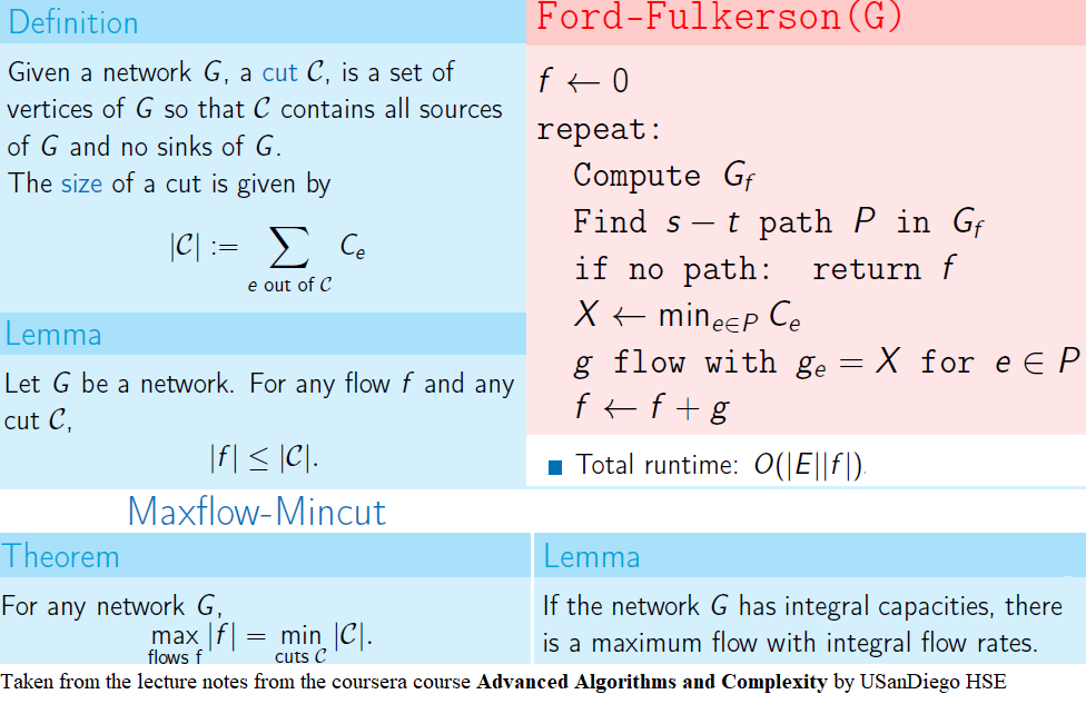
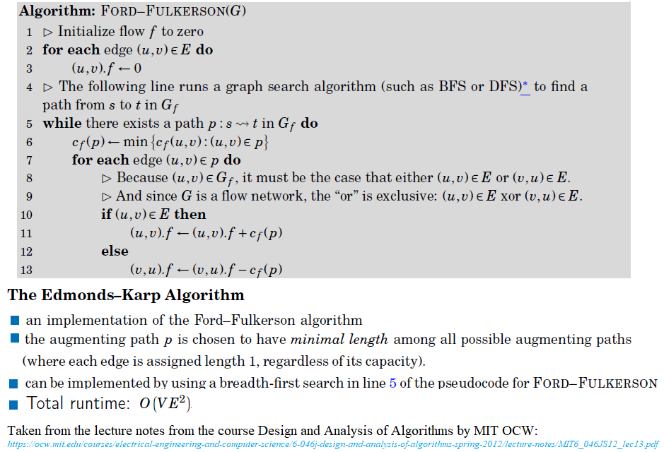
Ford-Fulkerson / Edmonds-Karp Algorithm for Max-flow
In this problem, we shall apply an algorithm for finding maximum flow in a network to determine how fast people can be evacuated from the given city.
The following animations show how the algorithm works. The red nodes represent the source and the sink in the network.

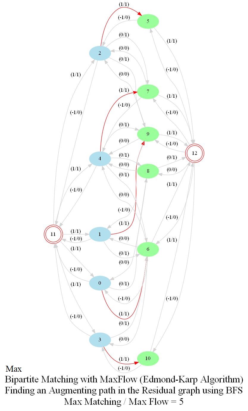
In this problem, we shall apply an algorithm for finding maximum matching in a bipartite graph to assign airline crews to flights in the most efficient way. Later we shall see how an Integer Linear Program (ILP) can be formulated to solve the bipartite matching problem and then solved with a MIP solver.
With Max-flow
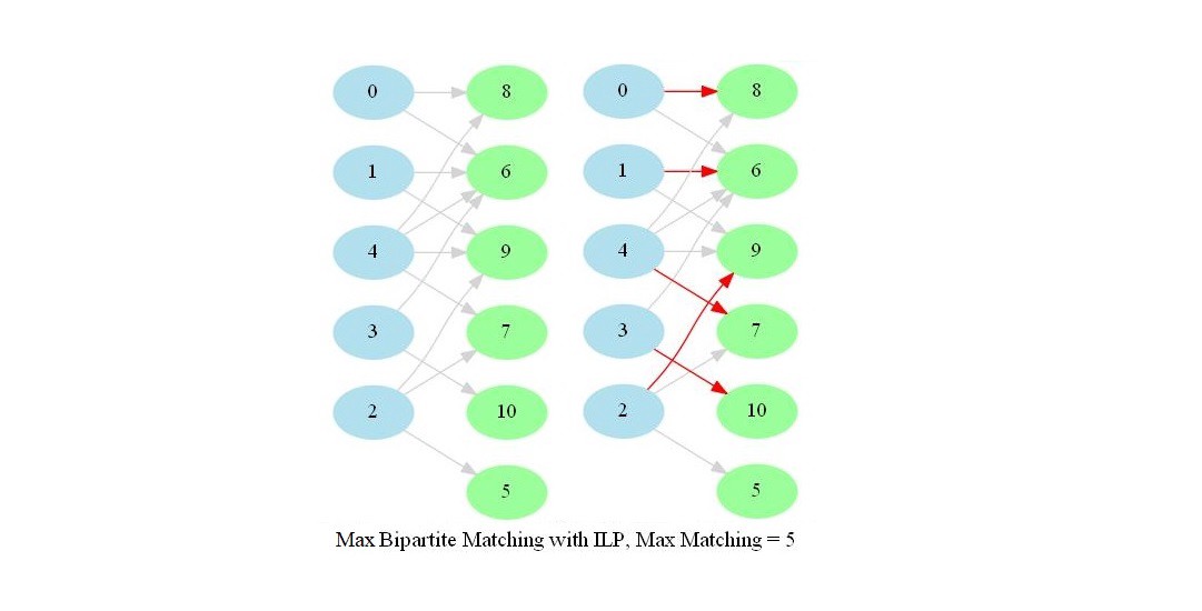
The following animations show how the algorithm finds the maximum matching for a few bipartite graphs (the blue and green nodes represent the self-edge-disjoint sets for the graph):
With Integer Linear Program
Using the mip package to solve the integer program and using a binary cost matrix c for the input bipartite graph G (where c[i,j]=1 iff i ∈ A and j ∈ B: A, B being disjoint vertex sets), the maximum bipartite matching problem can be solved with an ILP solver as shown in the following code snippet:
from mip import Model, xsum, maximize, BINARY

def mip_bipartite_matching(c):

   n, m = len(adj), len(adj[0])
   A, B = list(range(n)), list(range(m))

   model = Model()
   x = [[model.add_var(var_type=BINARY) for j in B] for i in A]

   model.objective = maximize(xsum(c[i][j]*x[i][j] \
                              for i in A for j in B))
   for i in A:
      model += xsum(x[i][j] for j in B) <= 1
   for j in B:
      model += xsum(x[i][j] for i in A) <= 1

   model.optimize()
   print(model.objective_value)
   return [(i,j) for i in A for j in B if x[i][j].x >= 0.99]
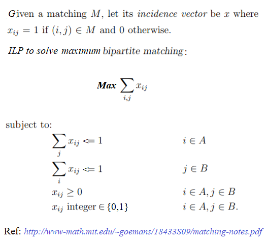
The ILP for the maximum bipartite matching problem can also be represented as follows in terms of the incidence matrix:
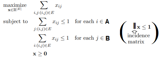
where the incidence matrix can be represented as follows, for the the above bipartite graph:
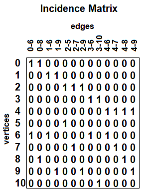
The above matrix can be shown to be totally unimodular (i.e., the determinant of any submatrix is either 0,-1 or 1, e.g., out of 215 submatrices of the above incidence matrix, 206 submatrices have determinant 0, 8 submatrices have deteminant 1 and 1 submatrix has determinat -1), implying that every basic feasible solution (hence the optimal solution too) for the LP will have integer values for every variable.
On the contrary, the solution obtained by the max-flow algorithm for the same input bipartite graph is shown follows:
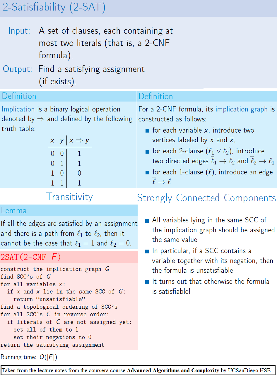
Solving 2-SAT problem and Integrated Circuit Design
VLSI or Very Large-Scale Integration is a process of creating an integrated circuit by combining thousands of transistors on a single chip. You want to design a single layer of an integrated circuit.
You know exactly what modules will be used in this layer, and which of them should be connected by wires. The wires will be all on the same layer, but they cannot intersect with each other. Also, each wire can only be bent once, in one of two directions — to the left or to the right. If you connect two modules with a wire, selecting the direction of bending uniquely defines the position of the wire. Of course, some positions of some pairs of wires lead to intersection of the wires, which is forbidden. You need to determine a position for each wire in such a way that no wires intersect.
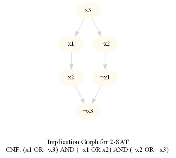
This problem can be reduced to 2-SAT problem — a special case of the SAT problem in which each clause contains exactly 2 variables. For each wire 𝑖, denote by 𝑥_𝑖 a binary variable which takes value 1 if the wire is bent to the right and 0 if the wire is bent to the left. For each 𝑖, 𝑥_𝑖 must be either 0 or 1.
Also, some pairs of wires intersect in some positions. For example, it could be so that if wire 1 is bent to the left and wire 2 is bent to the right, then they intersect. We want to write down a formula which is satisfied only if no wires intersect. In this case, we will add the clause (𝑥1 𝑂𝑅 𝑥2) to the formula which ensures that either 𝑥1 (the first wire is bent to the right) is true or 𝑥2 (the second wire is bent to the left) is true, and so the particular crossing when wire 1 is bent to the left AND wire 2 is bent to the right doesn’t happen whenever the formula is satisfied. We will add such a clause for each pair of wires and each pair of their positions if they intersect when put in those positions. Of course, if some pair of wires intersects in any pair of possible positions, we won’t be able to design a circuit. Your task is to determine whether it is possible, and if yes, determine the direction of bending for each of the wires.
The input represents a 2-CNF formula. We need to find a satisfying assignment to the formula if one exists, or report that the formula is not satisfiable otherwise.
The following animations show how the algorithm works.
Computing the Maximum Independent Set in a Tree
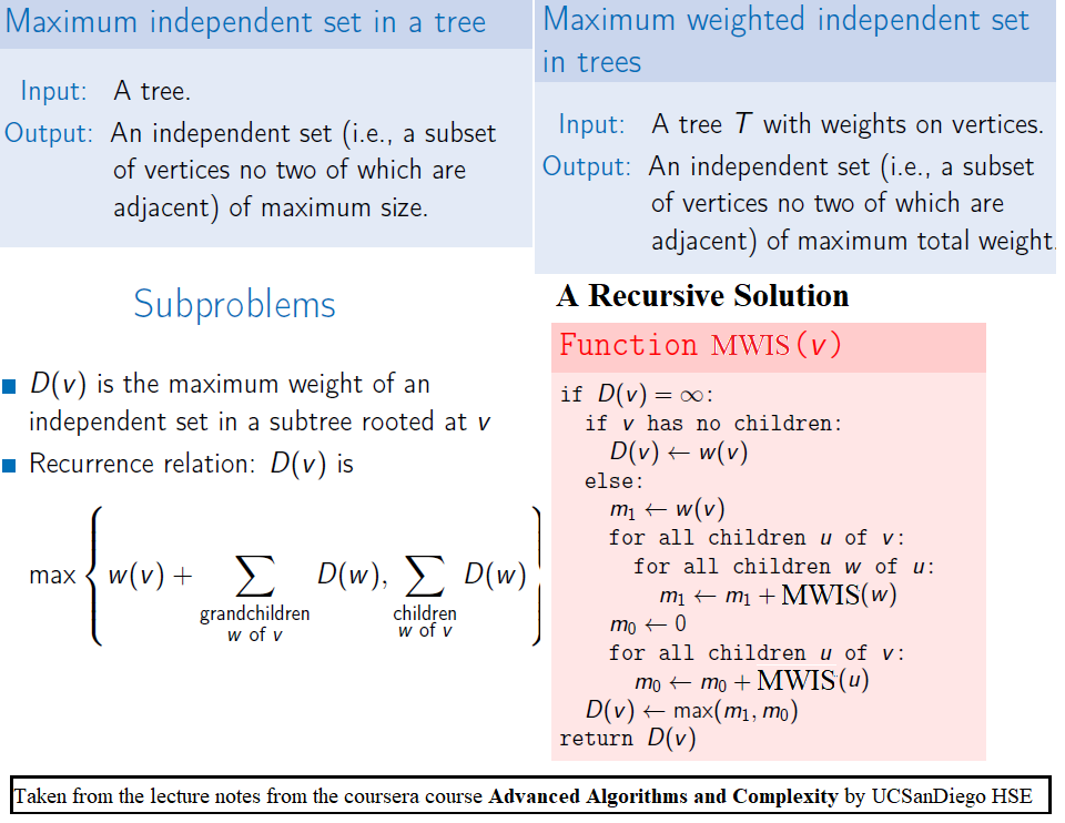
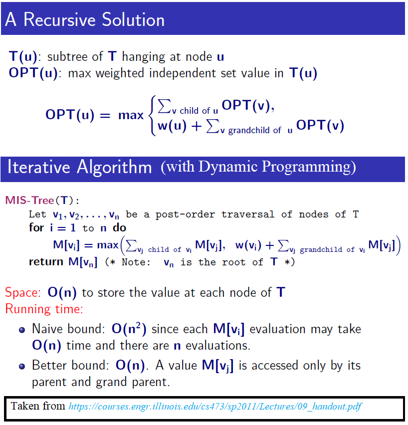
The following animations show how the dynamic programming algorithm computes the DP table (initialized to -1 for all nodes, as shown) and the corresponding maximum weighted independent sets for the subproblems and uses them to compute the MWIS of the entire tree. The pink nodes represent the nodes belonging to the maximum weighted independent set for a given subproblem (the root of the corresponding subtree is marked with double circles) and also for the final problem.
Computing the Convex Hull for a set of points in 2D
In this problem we shall implement Jarvis’ March gift wrapping algorithm to compute the convex hull for a given set of 2D points.
The following code snippet shows a python implementation of the algorithm. The points are assumed to be stored as list of (x,y) tuples.
import numpy as np

def cross_prod(p0, p1, p2):
    return (p1[0] - p0[0]) * (p2[1] - p0[1]) - \
           (p1[1] - p0[1]) * (p2[0] - p0[0])

def left_turn(p0, p1, p2):
    return cross_prod(p0, p1, p2) > 0

def convex_hull(points):
    n = len(points)
    # the first point
    _, p0 = min([((x, y), i) for i,(x,y) in  enumerate(points)])
    start_index = p0     chull = []
    while(True):
  	chull.append(p0)
 	p1 = (p0 + 1) % n #  make sure p1 != p0
	for p2 in range(n):
	   # if p2 is more counter-clockwise than
	   # current p1, then update p1
	   if left_turn(points[p0], points[p1], points[p2]):
		p1 = p2
	p0 = p1
	# came back to first point?
	if p0 == start_index:
	   break    return chull
The following animations show how the algorithm works.
The following animation shows a bad case for the algorithm where all the given points are on the convex hull.