Using PostgreSQL to Shape and Prepare Scientific Data
Today we are going to walk through some of the preliminary data shaping steps in data science using SQL in Postgres. I have a long history of working in data science, including my Masters Degree (in Forestry) and Ph.D. (in Ecology) and during this work I would often get raw data files that I had to get into shape to run analysis.
Whenever you start to do something new there is always some uncomfortableness. That “why is this so hard” feeling often stops me from trying something new, but not this time! I attempted to do most of my data prep and statistical analysis within PostgreSQL. I didn’t allow myself any copy and paste in google sheets nor could I use Python for scripting. I know this is hard core and in the end may not be the “best” way to do this. But if I didn’t force myself to do it, I would never understand what it could be like.
The Project
Next I needed to pick a modeling project. We have a few interesting data sets in the Crunchy Data Demo repository but nothing that looked good for statistical modeling. I thought about trying to find something a little more relevant to my life.
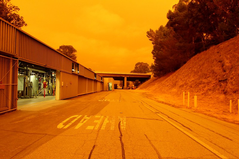
Photo by keppet on flickr
You may have noticed that we are having a few fires here in Northern California. Quite a few Crunchy folks live here. I'm in Santa Cruz (with a fire that was less than 7 miles away), Craig lives near Berkeley, Daniel and Will live in SF. We've compared notes on the sky (fun pic here), the amount of ash on cars, and PurpleAir values.
I thought it would be interesting to see if logistic regression could predict the probability of a fire based on the historical weather and fire patterns. All the details for how we obtained historical California fire data is here and here is the weather data.
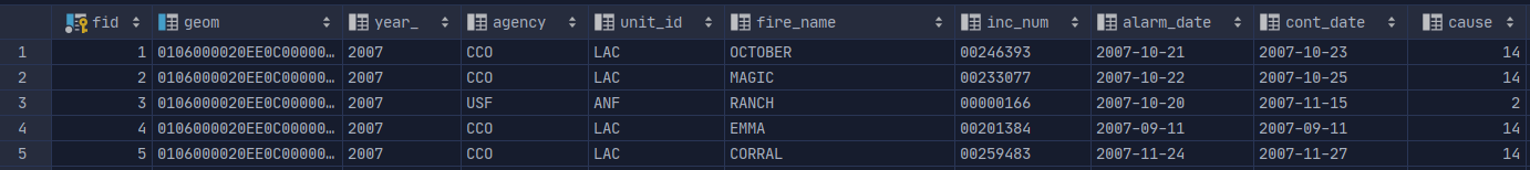
Here is a preview of the fire data:
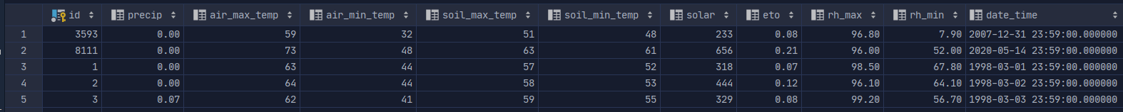
And here is a preview of the weather data:
Initial Import of Data
You can see on the pages above some of the initial cleaning we did. Most of it is minor though crucial things like renaming columns, taking a separate date and time column, and combining them into a timestamp, or changing the value on an obvious typo.
Let’s dig into the concatenating the date and time into a timestamp for the weather data (step 5). The old me would have put all the data in a spreadsheet and then used a concatenate function to put the two together. I would do one cell with the formula and then copy and paste into all the cells.
Instead, this is all we need:
UPDATE weather SET date_time = to_timestamp((date || ' ' || time || '-7'),
'YYYYMMDD HH24:MI');
One of the obvious advantages you should see right away is that we only have one line of code to accomplish what would take several manual steps. Since it’s in code if we need to reimport the data or modify it for another data set, we just have to reuse this line. We could even use this as part of an automated script.
The other thing you should notice is that we were able to actually add a timezone to the data (the -7). And finally, we were able to act on the data as a whole unit. That means we do the operation all at once without fat-fingering the data or forgetting to paste some sort of rows. The data stays together and all the operations happen at “the same time”. If we wanted to be even more careful we could have wrapped the statement in a transaction.
Subsetting Our Data
The first thing we are going to do to shape our data is subset the fires. Our weather station is in Northern California and so it probably doesn’t make sense to try and predict Southern California fire probability given weather in the north. This is again a one liner to subset our data:
SELECT fire19.* INTO ncalfire FROM fire19, fire19_region WHERE
*st_covers\*(fire19_region.geom, fire19.geom) AND fire19_region.region =
'Northern';
We selected all the columns from the original data where the Northern Region
covers all the fire data. We use ST_Covers rather than ST_Contains because
of some
unexpected behaviour
in ST_Contains. By using st_covers, our operation will not include any fires
whose boundaries go outside the Northern Region, for example if the fire spread
into Oregon.
Getting ready for Logistic Regression
Logistic regression needs the response variable (did a fire happen on that day), be coded as a 1 = fire happened, 0 = no fire. When I started to examine the data, as I should have known based on living in California, multiple fires can start on the same day. So we need to aggregate data from multiple days into a single entry. With SQL we don’t have to lose any information. Here is the one line that does what we need:
WITH grouped_fire AS (
 SELECT alarm_date, count(*) as numfires, string_agg(fire_name, ', ') AS names,

*st_collect*(geom)::geometry(geometrycollection, 3310) AS geom FROM ncalfire
GROUP BY alarm_date
 )
SELECT w.*, grouped_fire.\*, 1 AS hasfire INTO fire_weather FROM weather w, grouped_fire
WHERE grouped_fire.alarm_date = w.date_time::date;
So the first part of this query starting WITH grouped_fires until the ) is
called
a CTE
or common table expression. We do all our aggregation in the CTE
based on alarm_date (specified by the GROUP BY alarm_date). Our output will
be for each alarm date:
- Return the number of fires that happened on that day.
- Aggregated all the strings for the fire names into one string separated by “,” (we could have also used an an array of string).
- Collect the geometries of all the different fires on that day into one geometry collection.
Now we can use the information from the CTE like a table in the second part of
the query. In the next part we grab all the columns from the CTE along with all
the columns in the original table and then we just put a 1 in for all entries in
an output column named hasfire.
As a side note, I am a big fan of bringing clarity to boolean columns by
prefixing them with is or has so you know what the true condition means.
Then we join the CTE date to the original table by matching dates. We truncate
the timestamp column by casting it to a date. Notice we are selecting into a new
table and the output of this command will actually go into a table rather than
showing on the screen. With that we now have a table with all the weather data,
dates of fires, and a 1 in the hasfire column.
Fixing our Geometry
You will notice above we had to make a geometrycollection to group the fires geometries together. Most desktop and other GIS software don’t know what to do with a geometrycollection geometry type. To fix this problem we are going to cast the geometries to multipolygons. A multipolygon allows a single row to have multiple polygons. The easiest example of this is a town or property that includes islands. A multipolygon allows the town, along with its islands, to be seen as a single entry in the table. Here is the call we use:
ALTER TABLE fire_weather ALTER COLUMN geom type geometry(multipolygon,3310)
USING st_collectionextract(geom, 3);
ST_collectionextract
takes a multigeometry and collects all the geometries you ask for and returns a
multigeometry of the requested type. The 3 in st_collectionextract is the
“magic number” meaning polygons
Creating our non-fire data
We created our fire data and fixed it’s geometry. Now we have to go back to the weather data and assign 0 to all the days where there was no fire:
WITH non*fire_weather AS (
SELECT weather.* FROM weather WHERE id NOT IN (SELECT id FROM fire*weather)
)
SELECT non_fire_weather.*, null::date AS alarm_date, 0::bigint AS numfires,
null::text AS names, null::geometry(MultiPolygon,3310) AS geom, 0 AS hasfire
INTO non_fire_weather FROM non_fire_weather;
Again we are going to start with a CTE but this time the first query is used to
find all the days that are NOT in the new fire + weather table above. This gives
us a “table” with only weather data on days where a fire did not occur. Then in
the second part of the query we add in all the columns that we added to our
fire_weather table. Finally we put the results into a new table called
non_fire_weather.
Now we combine the fire_weather and non_fire weather tables into one master
table called alldata:
SELECT _ INTO alldata FROM non_fire_weather UNION SELECT _ FROM fire_weather;
We did this merging with the full data set in case we want to do other types of analyses with this data. For example, we actually have counts of fire on days and we also have total area of fire burned (from the polygons). These variables might lead to other interesting analysis in the future.
Wrap Up
Let’s wrap up and look at all the good work we were able to do using SQL for data science. We took some tables imported from raw data, turned dates and time into more usable formats, aggregated the fire events, kept the geometries intact, created a code for event versus not event, and created a large master data set.
All of this was done with lines of code, no manual steps. Doing our data shaping this way makes our process easily repeatable if we need to do it again. We could actually put it in a script and automate the importing of new data. On a personal note, it makes my life so easy if I need to create a new version of the dataset or import the data to a new server.
I hope you found this code and the examples useful in your data science work (here is the github repo for it). What is your experience with using SQL to shape your data before doing analysis? Do you have some tips or tricks you would like to share? Leave us comment on the Crunchy Data twitter account. Have fun with your analysis and code on!
Cover image By Annette Spithoven, NL
