I got a little ahead of myself with the title of my last post, “Everything you want to know about subplots in Python’s Matplotlib”. While the information in that post can allow you to do quite a lot, there is in fact more that you might want to know. In this post I’ll go over two more subplot tools that are helpful for designing informative and attractive subplots. First, I’ll discuss working with colorbars, a seemly minor task that can be quite time consuming. Then I’ll discuss a brand new feature of Matplotlib, the subplot_mosaic interface. This feature is still in its testing phase, but will likely be the new standard for making subplots in the future.

Formatting colorbars with constrained_layout

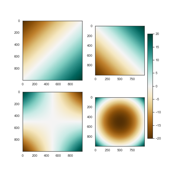
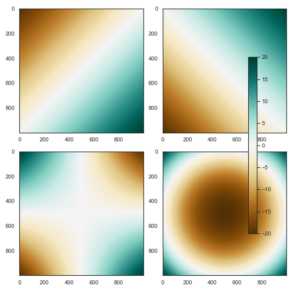
Colorbars play an important role in data visualization. Often, you may use a common color to link multiple views of the same data set, or contrast two data sets. Making a colorbar in matplotlib is fairly easy, but unless you use the right tools, making the colorbar fit into the overall graphic can be unexpectedly difficult. Here’s an example of creating a single colorbar for four different subplots. The fig.colorbar() function, allows you to easily add a colorbar to the set of subplots. Unfortunately, with the default settings, this code will shrink two subplots disproportionately.

from matplotlib import pyplot as plt
from mpl_toolkits.axes_grid1 import make_axes_locatable
import numpy as np

# create some sample data
x = np.linspace(-10.0, 10.0, 1000)
y = np.linspace(-10.0, 10.0, 1000)
X, Y = np.meshgrid(x, y)
Z1 = X + Y
Z2 = X - Y
Z3 = X*Y
Z4 = X**2+Y**2

# create a figure object
fig, axes = plt.subplots(2,2, figsize=(8,8))
im1 = axes[0,0].imshow(Z1, cmap='BrBG')
im2 = axes[0,1].imshow(Z2, cmap='BrBG')
im3 = axes[1,0].imshow(Z3, cmap='BrBG')
im4 = axes[1,1].imshow(Z4, cmap='BrBG')

cbar = fig.colorbar(im1, ax=axes[:, 1], shrink=0.8)

One way you may attempt to fix this could be to use the tight_layout() function, which can help align subplots. This will make things worse however, because the colorbar confuses the algorithm that tight_layout uses to arrange the axes objects. The result will look like this (and produce an warning output):

Luckily, there is an alternative to tight_layout, called constrained_layout, which uses a constrained solver to optimize subplot placement. Constrained layout should be called during the creation of the figure object, as demonstrated below. Applying constrained layout to this set of subplots fixes the error and creates a nice looking set of plots.

# create a figure object
fig, axes = plt.subplots(2,2, figsize=(8,8), constrained_layout=True)
im1 = axes[0,0].imshow(Z1, cmap='BrBG')
im2 = axes[0,1].imshow(Z2, cmap='BrBG')
im3 = axes[1,0].imshow(Z3, cmap='BrBG')
im4 = axes[1,1].imshow(Z4, cmap='BrBG')

cbar = fig.colorbar(im1, ax=axes[:, 1], shrink=0.8)

I should note that we can edit the colorbar axes object just like any of the other axes objects, adding labels, adjusting the tick marks etc. For more on colorbars, see the documentation here.

The subplot_mosaic interface

In my last post I discussed the Gridspec interface, which allows you to manually configure custom grid of subplots. While Gridspec can create complex configurations of subplots, manually adjusting the grid can become complicated for complex layouts. Matplotlib recently introduced a new feature, subplot_mosaic, which allows a more intuitive interface for configuring subplots. The subplot_mosaic has a simple and streamlined interface that allows you to easily lay out subplots, then stores these subplots as a dictionary. It’s important to note that this feature is still in testing and (at the time of this posting) is not currently supported by many distributions such as Anaconda. For more examples and full documentation, see the official release page.