There are various ways that we can approach the analysis of a past database performance problem. The initial steps usually differ based on their scope. Is it limited to a certain SQL/process/task, or is it perceived as a database-wide slowdown? Additionally, is it occurring at the moment, or is it an event that occurred in the past? In case the starting scope of analysis is database-wide, mining the Automatic Workload Repository (AWR) is one of the methods we can use to obtain historical performance trends. However, not all customers have access to it, either because it requires the Diagnostics Pack license on Enterprise Edition, or because they are running Oracle Standard Edition, where it's not present. In such cases, we can still use Statspack as a free alternative to AWR, even though it's not as sophisticated. One of Statspack's shortcomings is it doesn't store Active Session History data, which we can use to drill-down into the activity of particular sessions over time. With Statspack we're missing this session-level granularity. In this post, I'm going to present a script I use to get an overview of the workload dynamics of a database querying the Statspack repository. There's also an AWR counterpart, as I'll mention later in the post.
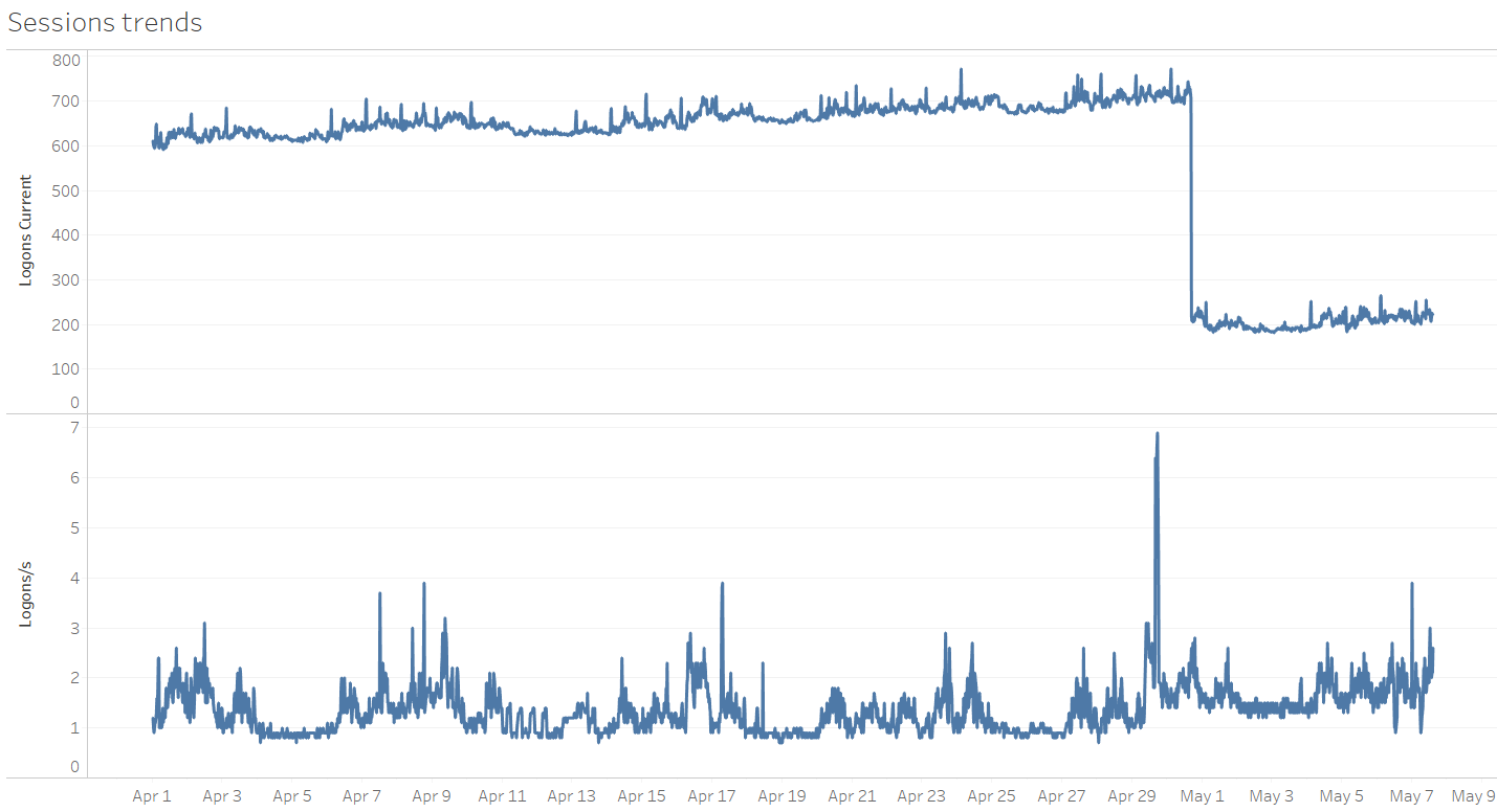
 A final example from a different server, but still related to connection management. Detecting a large drop in the number of established sessions and correlating with the number of logins per second:
statspack_load_trends.sql
1. Script's Properties
Let's summarize the script's main properties:- It queries the Statspack repository directly and doesn't create any (temporary) objects, nor relies on any pre-created Statspack reports.
- We can use it to analyze a Statspack repository imported from another DB, containing data with a different DBID as the DB hosting the repository.
- We can analyze a period spanning instance restart(s). The script considers only adjacent snapshot pairs having the same startup_time value. In this case, "adjacent" denotes two snapshots which belong to the same [DBID, instance number] pair, and which SNAP_IDs are closest to each other when ordered. That's just to emphasize that the difference between two consecutive SNAP_IDs is not always one (think RAC with cached sequence values, an instance restart, or pressure on the shared pool).
2. Purpose
The script provides a quick high-level overview of the DB workload dynamics. It reports a combination of historical OS utilization statistics (stats$osstat), system time model statistics (stats$sys_time_model), and aggregated instance-level statistics (stats$sysstat) for a given period. Currently, it doesn't query stats$system_event for wait event details. Several time-based metrics are presented in a form of Average Active Sessions (AAS), calculated by simply dividing the observed time-based metric by the elapsed time in the observed period. You can download the script here, and its AWR counterpart is available here. Before running the AWR version, make sure the database has the Diagnostics Pack license. The following explanation applies to both scripts. Note: I got the idea for this script from various AWR mining scripts in Chapter 5 (Sizing Exadata) from the "Oracle Exadata Recipes: A Problem-Solution Approach" book. Additionally, the idea to calculate and display CPU core-normalized values for some of the CPU usage statistics originates from John Beresniewicz's AWR1page project.3. Calculating CPU Capacity
The script considers the number of CPU cores, and not threads (in case hyperthreading is enabled) to calculate the number of CPU seconds between two Statspack snapshots. Various publications explain the reasons for this approach, but to summarize: Depending on the workload type, hyperthreading can provide up to approx. 30% higher CPU throughput compared to non-hyperthread mode. When the number of processes running on CPU approach the number of CPU cores, the system might become CPU saturated/over-subscribed. At that point, its response time becomes unpredictable, and additional workload decreases the amount of useful work performed by the system.4. Usage
The script produces a very wide output, so I recommend spooling it out to a file for easier viewing. Because Statspack tables have public synonyms, any user that has permission to select from the repository tables can run it. Note: I've seen the script fail with errors like "ORA-00936: missing expression," or "ORA-01722: invalid number" when used on databases running with cursor_sharing=FORCE. To avoid the error, I included the /*+ cursor_sharing_exact*/ hint in the script's SELECT statement. Setting cursor_sharing=EXACT at the session-level is also a valid alternative.SQL> spool load_trends.txt SQL> @statspack_load_trends.sqlFirst, we provide the DBID and instance number we want to analyze. If we don't provide an instance number, all of the instances for the provided DBID are considered:
Instances in this Statspack schema
 ~~~~~~~~~~~~~~~~~~~~~~~~~~~~~~~~~~
  DB Id |Inst Num|DB Name |Instance |Host
 -----------|--------|------------|------------|-------------
  1558102526| 1|ORCL |orcl1 |ol7-122-rac1
  1558102526| 2|ORCL |orcl2 |ol7-122-rac2


 Enter DBID to analyze - default "1558102526" : /* enter DBID to analyze */
 Enter instance number or "all" to analyze all instancs for DBID = 1558102526 - default "all" : /* report data for a specific RAC instance or all of them */
Next, we provide a time range to analyze.
5. Sample Output
Let's check what the output looks like. Due to its width, and to fit the blog format, it's segmented in several sections. Also, due to some (temporary) blog formatting limitations, I recommend viewing wide code sections by clicking "Open code in new window."- "CPU #Cores;#Threads": The number of CPU cores and threads (in case of enabled hyperthreading) reported by the OS.
- "Tot CPU Time Avail [Cores] (s)": The number of CPU seconds available between the two analyzed snapshots based on the number of CPU cores.
Instance|Snap ID |Begin Snap |End Snap |Elapsed| CPU| Tot CPU Time| Number|start-end |Time |Time | Mins|#Cores;#Threads|Avail [Cores] (s)| --------|---------------|---------------|---------------|-------|---------------|-----------------| 1|19195-19196 |16-APR-20 17:00|16-APR-20 18:00| 59.98| 24; 48| 86,376.00| |19196-19197 |16-APR-20 18:00|16-APR-20 19:00| 60.00| 24; 48| 86,400.00| |19197-19198 |16-APR-20 19:00|16-APR-20 20:00| 60.00| 24; 48| 86,400.00| |19198-19199 |16-APR-20 20:00|16-APR-20 21:00| 60.02| 24; 48| 86,424.00| |19199-19200 |16-APR-20 21:00|16-APR-20 22:00| 59.98| 24; 48| 86,376.00|Note: One hour between snapshots is probably excessive, but that's beyond the scope of this post.
Time Model Statistics: stats$sys_time_model
The next section reports the time spent in the database in the form of Average Active Sessions (AAS). For completeness, and to better understand what the figures represent, I'm including how various statistics from stats$sys_time_model are related:DB time = CPU + Wait time spent by foreground sessions background elapsed time = CPU + Wait time spent by background sessions DB CPU = CPU time spent by foreground sessions background cpu time = CPU time spent by background sessionsConsidering the above, we can calculate the AAS figures as follows:
 Total AAS = ("DB time" + "background elapsed time")/elapsed_time
 Total AAS on CPU = ("DB CPU" + "background cpu time")/elapsed_time

 FG AAS = "DB time" / elapsed_time
 BG AAS = "background elapsed time" / elapsed_time

 FG AAS on CPU = "DB CPU" / elapsed_time
 BG AAS on CPU = "background cpu time" / elapsed_time

 Total AAS in wait = ("Total AAS" - "Total AAS on CPU") / elapsed_time

 FG AAS in wait = ("DB time" - "DB CPU") / elapsed_time
 BG AAS in wait = ("background elapsed time" - "background cpu time") / elapsed_time
Columns reporting CPU-related figures display two values: The "usual" AAS value, and the "core-normalized Average Active Sessions" value, using the acronym "NPC". If the core-normalized value approaches (or even crosses) the value of "1," the system could potentially be CPU saturated:
- "AAS [FG+BG]": The number of AAS considering foreground and background sessions.
- "AAS [FG]": The number of AAS considering foreground sessions only.
- "AAS [BG]": The number of AAS considering background sessions only.
- "AAS on CPU [FG+BG]": The number of AAS on CPU considering foreground and background sessions, followed by core-normalized AAS on CPU (NPC).
- "AAS on CPU [FG]": Same as above, though only considering foreground sessions.
- "AAS on CPU [BG]": Same as above, though only considering background sessions.
 AAS| AAS| AAS|AAS on CPU| AAS on CPU|AAS on |AAS on CPU|AAS on |AAS on CPU| AAS wait| AAS wait| AAS wait| |
  [FG+BG]| [FG]| [BG]|[FG+BG] |[FG+BG] NPC|CPU [FG]| [FG] NPC|CPU [BG]|[BG] NPC | [FG+BG]| [FG]| [BG]|AAS RMAN CPU |
 ---------|---------|---------|----------|-----------|--------|----------|--------|----------|---------|---------|---------|-------------|
  96.4| 94.3| 2.0| 8.5| 0.4| 8.3| 0.3| 0.2| 0.0| 87.9| 86.0| 1.9| 0.0|
  32.9| 31.6| 1.3| 10.3| 0.4| 10.1| 0.4| 0.2| 0.0| 22.5| 21.4| 1.1| 0.0|
  59.4| 58.9| 0.6| 23.3| 1.0| 23.2| 1.0| 0.1| 0.0| 36.2| 35.7| 0.5| 0.0|
  13.3| 12.9| 0.5| 5.8| 0.2| 5.7| 0.2| 0.1| 0.0| 7.5| 7.1| 0.4| 0.0|
  23.0| 22.2| 0.8| 6.0| 0.3| 5.9| 0.2| 0.1| 0.0| 17.0| 16.3| 0.7| 0.0|
The first line reports 94.3 foreground AAS, out of which only 8.3 were on CPU, and 86 were in various waits. Looking at the third line, the situation changes, as out of the 58.9 AAS, 23.3 were on CPU, and 35.7 in waits. Checking the per-CPU-core-normalized value, we see it reports 1, which means the machine might be approaching or has already crossed CPU saturation. We also see that there was no RMAN activity occurring during that time. Background processes also spent most of their time in waits, rather than on CPU. For convenience, we have displayed the number of seconds consumed by foreground sessions, breaking them further down into CPU and wait components, and reporting the relative percentages. This is basically the same information we saw in the previous section, just expressed as time instead of AAS:
 DB Time (s) DB CPU (s) |
 [FG CPU+WAIT] = [FG CPU] + [FG WAIT] |
 ---------------------------------------------------------|
  339,555.62 = 29,924.51 9% + 309,631.11 91% |
  113,683.70 = 36,469.52 32% + 77,214.18 68% |
  211,880.46 = 83,404.47 39% + 128,475.99 61% |
  46,325.13 = 20,692.78 45% + 25,632.35 55% |
  79,966.07 = 21,274.38 27% + 58,691.69 73% |
OS Statistics - stats$osstat
Next, OS statistics from stats$osstat are displayed. "Tot OS Load@end_snap" is the recorded OS load at the time of the end snapshot creation. The other four columns represent Average Active Processes (AAP), which is simply the measured time of each named statistic divided by elapsed time in the observed period. Similarly, as above, the normalized value per core is also reported here for the BUSY statistic (sum of USER+SYS). The meaning is the same; If the value approaches 1, the system might be CPU saturated. In our sample report, the third line reports 23.9 processes on CPU, or 1 per CPU core (that's considering all the OS processes, not only Oracle's). That also correlates with the "AAS on CPU [FG+BG]" figure in the third line we saw in the above snippet. Because in this particular case the machine is dedicated to one Oracle instance, it used all of the available CPU:Tot OS| |AAP OS | AAP OS| AAP OS| AAP OS| Load@end_snap|AAP OS BUSY|BUSY NPC| USER| SYS| IOWAIT| -------------|-----------|--------|---------|---------|---------| 37.0| 9.2| 0.4| 8.2| 0.9| 12.1| 76.8| 10.8| 0.4| 9.8| 0.9| 5.3| 9.4| 23.9| 1.0| 22.9| 0.9| 2.3| 4.3| 6.2| 0.3| 5.7| 0.5| 1.4| 4.8| 6.4| 0.3| 5.6| 0.7| 4.7|
System Statistics: stats$sysstat
Finally, stats$sysstat reports various system statistics. I won’t describe their meaning because that's beyond the scope of this post. It's worth noting that apart from "Logons Current," almost all other statistics are expressed in units of work per second. The only exceptions are statistics related to parallel operations. Because their usage usually pertains to "heavy-duty" DDL/DML tasks, we don't expect to see many such operations per second. Thus, the whole snapshot interval seems a more appropriate time-frame to report the number of occurrences of such events.Logons| | User| |SQL*Net roundtrips|SQL*Net roundtrips| Bytes received via| Bytes sent via| Bytes received via| Current|Logons/s| calls/s| Executes/s| to/from client/s| to/from dblink/s|SQL*Net from client/s|SQL*Net to client/s|SQL*Net from dblink/s| ----------|--------|----------|------------|------------------|------------------|---------------------|-------------------|---------------------| 556.0| 9.5| 872.9| 692.2| 723.0| 4,575.6| 1,846,238.6| 6,305,967.2| 1,177,004.3| 527.0| 16.2| 1,008.0| 639.4| 828.5| 5,773.2| 2,462,067.1| 7,760,807.5| 1,453,024.0| 607.0| 18.5| 738.8| 588.3| 556.1| 5,618.1| 1,986,647.1| 3,644,026.9| 1,448,627.4| 427.0| 9.2| 873.3| 910.0| 716.4| 5,972.3| 2,691,244.6| 4,067,039.1| 1,532,389.7| 418.0| 7.4| 719.9| 627.8| 588.5| 7,471.6| 2,564,916.7| 3,773,344.1| 1,852,806.9| Bytes sent via|Cluster wait|Session logical| DB block| Consistent| Consistent reads | Physical| Physical|Physical read|Physical write| SQL*Net to dblink/s| time/s| reads/s| changes/s| changes/sec|undo rec applied/s| reads/s| writes/s|IO requests/s| IO requests/s| -------------------|------------|---------------|--------------|--------------|------------------|----------|----------|-------------|--------------| 576,510.8| 0.0| 339,009.8| 31,353.8| 3,062.0| 4,002.4| 47,349.4| 1,879.1| 2,621.5| 448.5| 726,935.7| 0.0| 487,469.9| 48,874.4| 487.3| 563.9| 31,277.7| 2,127.6| 5,021.6| 526.8| 707,648.6| 0.0| 343,665.8| 38,862.0| 379.4| 362.9| 37,057.7| 777.7| 1,949.2| 265.2| 751,698.7| 0.0| 288,724.2| 26,163.7| 618.0| 435.8| 14,001.6| 823.3| 828.5| 274.1| 940,096.3| 0.0| 335,631.4| 24,500.0| 198.5| 211.9| 53,625.8| 638.2| 2,451.6| 227.5| Parses| Hard| Parse| Parse| User| User| Redo size| Redo| Rollback changes| total/s| parses/s|describe/s|failures/s| commits/s|rollbacks/s| bytes/s| writes/s|undo records applied/s| ----------|----------|----------|----------|----------|-----------|--------------|--------------|----------------------| 142.0| 103.9| 0.0| 0.0| 158.2| 0.8| 46,951,095.1| 137.8| 0.1| 143.4| 100.1| 0.0| 0.3| 155.0| 0.8| 49,017,168.1| 170.3| 1.2| 135.9| 89.2| 0.0| 0.1| 143.3| 0.8| 11,513,858.2| 149.7| 0.1| 141.1| 109.8| 0.0| 0.0| 284.4| 0.8| 9,513,089.1| 226.2| 0.1| 123.0| 93.4| 0.0| 0.0| 175.5| 0.9| 7,462,206.6| 169.3| 0.3| Queries| DML statements| PX oper not|PX oper downgraded|PX oper downgraded|PX oper downgraded|PX oper downgraded|PX oper downgraded parallelized/Total|parallelized/Total|downgraded/Total| to serial/Total|75 to 99 pct/Total|50 to 75 pct/Total|25 to 50 pct/Total| 1 to 25 pct/Total ------------------|------------------|----------------|------------------|------------------|------------------|------------------|------------------ 1,912.0| 3.0| 1,989.0| 38.0| 0.0| 1.0| 4.0| 1.0 2,450.0| 6.0| 2,551.0| 10.0| 0.0| 0.0| 0.0| 0.0 2,477.0| 13.0| 2,584.0| 9.0| 0.0| 0.0| 0.0| 0.0 1,553.0| 3.0| 1,646.0| 9.0| 0.0| 0.0| 0.0| 0.0 1,390.0| 2.0| 1,487.0| 8.0| 0.0| 0.0| 0.0| 0.0
6. Visualizing Results
When comparing a period where there was an issue to one where the database was running fine, or also when just checking for trends, it's more convenient to plot the results. That's an easy way to get an overview of how certain metrics changed over time, or how do they compare across nodes on a RAC database. To ease that task, the two scripts contain two ways of formatting columns: One for plotting/charting purposes, and one displaying column headings on two lines for a more user-friendly format (the format used in the above descriptions). Based on the needs, the appropriate block of column formatting commands has to be uncommented in the script. You can plot results using a third-party utility, such as Tableau, which is used to produce graphs in the following sections.CPU Usage Distribution and Limits Across Nodes
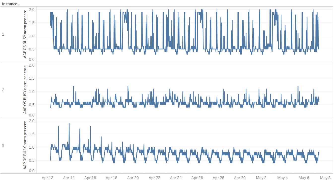
The graph below represents the average number of OS processes on CPU, normalized to the CPU core count for each of the three nodes on a RAC system. As noted above, when the normalized value per core crosses the value of "1," the host might be oversubscribed on CPU. Nodes 2 and 3 are usually below the value of 1. However, spikes in usage on node 1 might require further investigation. Also, there seems to be an imbalance in CPU usage across nodes:
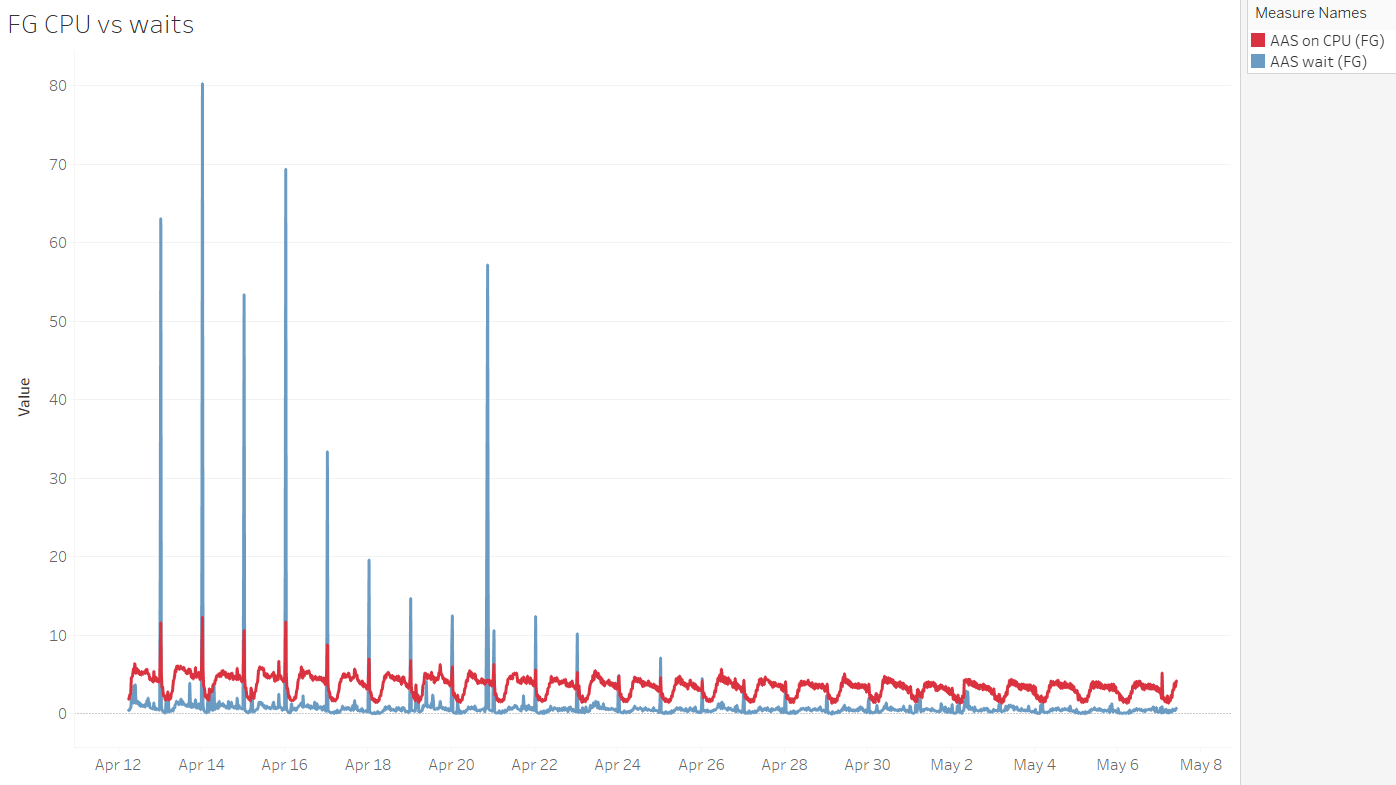
Breakdown of Foreground and Background Sessions on CPU and Wait Components, Expressed as AAS
When investigating a problematic time period, we can quickly get a high-level overview of the relation between CPU and waits experienced by foreground and background sessions: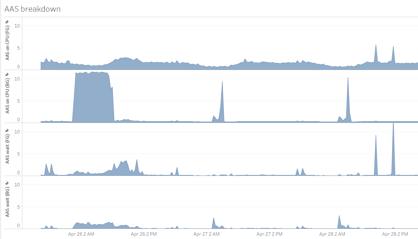
Observing Waits After Applying a Fix to Reduce Them
After applying "a fix" on April 16th, the time spent waiting by foreground sessions decreased substantially. CPU demand also decreased.
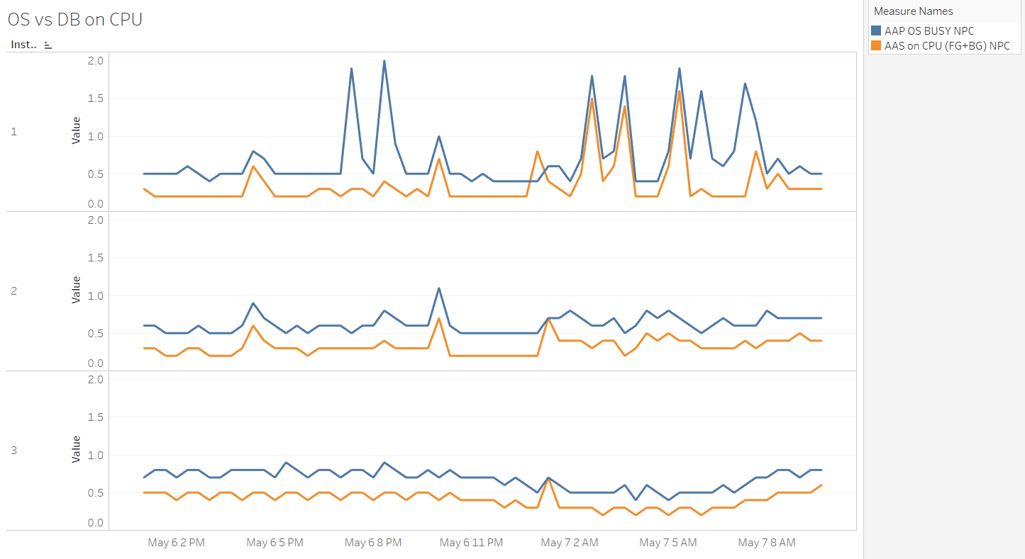
Comparing the Number of AAS on CPU Normalized to CPU Core Count at the OS and DB Level on a Three-Node RAC DB
The observed DB isn't using all/most of the CPU available on the nodes, and there's "something else" using it at the OS level. That's visible on the graph for node 1, between May 6th at 7-9 PM, where CPU usage at the OS level increased, but that was not the case for DB sessions. Additionally, because we have the normalized per CPU core value displayed, we can see that node 1 crosses the value of 1 quite often.
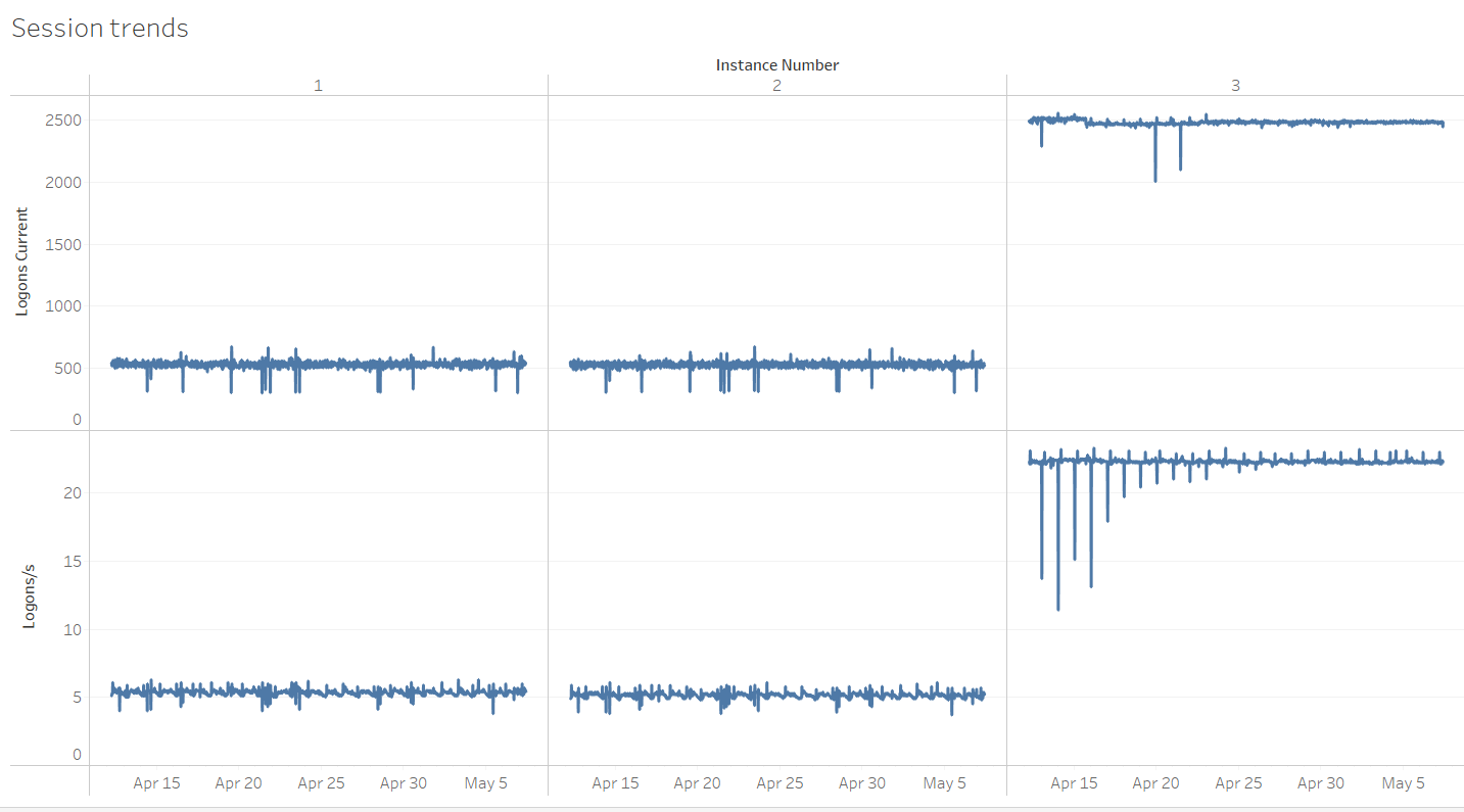
Logons per Second and Number of Logged-in Sessions per Node
RAC nodes 1 and 2 already have a relatively high number of Logons per second at ~5, whereas node 3 has this even higher at ~23. Additionally, there's a large imbalance in the number of established sessions on node 3 compared to nodes 1 and 2. Because each node has 8 physical cores (not visible from the below graphs), the ~2500 established sessions represent a potential risk should too many of them try to become active at the same time. Overall it seems a connection pooling review is in place for this system. A final example from a different server, but still related to connection management. Detecting a large drop in the number of established sessions and correlating with the number of logins per second:
7. Other Mining Tools
Some time ago, Maris Elsins published a post describing a set of handy scripts to mine the AWR repository. Make sure to check it out! To conclude, here's a list of some free mining utilities. These are mostly created for AWR, but some are for Statspack. Some of them parse a pre-created set of AWR/Statspack reports. Others connect directly to the database and extract/analyze data from there. The script presented in this post might not offer the same functionality as those utilities. However, for some of my use-cases, it complemented them by providing a customized set of pre-calculated workload related figures.- https://github.com/LucaCanali/PerfSheet4
- https://github.com/sqldb360/sqldb360
- https://flashdba.com/database/useful-scripts/awr-parser/
- https://github.com/sfurlong/visual-awr
- https://github.com/ora600pl/statspack_scripts
8. Display performance metrics at SQL Level
In the
next post, I'll present the
statspack_top_sqls.sql script which provides a more detailed breakdown of SQL performance metrics for a given time period by querying the Statspack repository.

