It’s funny how similar ideas pop up in different branches of mathematics. Calculus, for instance, is built around metric spaces (or, more generally, Banach spaces) and measures. A limit of a sequence is defined by points getting closer and closer together. An integral is an area under a curve. In category theory, though, we don’t talk about distances or areas (except for Lawvere’s take on metric spaces), and yet we have the abstract notion of a limit, and we use integral notation for ends. The similarities are uncanny.
This blog post was inspired by my trying to understand the idea behind the Freyd’s adjoint functor theorem. It can be expressed as a colimit over a comma category, which is a special case of a Grothendieck fibration. To understand it, though, I had to get a better handle on weighted colimits which, as I learned, were even more general than Kan extensions.
Category of elements as coend
Grothendieck fibration is like splitting a category in two orthogonal directions, the base and the fiber. Fiber may vary from object to object (as in dependent types, which are indeed modeled as fibrations).
The simplest example of a Grothendieck fibration is the category of elements, in which fibers are simply sets. Of course, a set is also a category—a discrete category with no morphisms between elements, except for compulsory identity morphisms. A category of elements is built on top of a category 

Such a functor is traditionally called a copresheaf (this construction works also on presheaves, 


A morphism from 


There is an obvious projection functor that forgets the second component of the pair

(In fact, a general Grothendieck fibration starts with a projection functor.)
You will often see the category of elements written using integral notation. An integral, after all, is a gigantic sum of tiny slices. Similarly, objects of the category of elements form a gigantic sum (disjoint union) of sets 

However, this notation conflicts with the one for conical colimits so, following Fosco Loregian, I’ll write the category of elements as

An interesting specialization of a category of elements is a comma category. It’s the category 


You’ll mostly see integral notation in the context of ends and coends. A coend of a profunctor is like a trace of a matrix: it’s a sum (a coproduct) of diagonal elements. But (co-)end notation may also be used for (co-)limits. Using the trace analogy, if you fill rows of a matrix with copies of the same vector, the trace will be the sum of the components of the vector. Similarly, you can construct a profunctor from a functor by repeating the same functor for every value of the first argument 

The coend over this profunctor is the colimit of the functor, a colimit being a generalization of the sum. By slight abuse of notation we write it as

This kind of colimit is called conical, as opposed to what we are going to discuss next.
Weighted colimit as coend
A colimit is a universal cocone under a diagram. A diagram is a bunch of objects and morphisms in 


For any given indexing object 


)](https://s0.wp.com/latex.php?latex=%5B%5Cmathcal%7BJ%7D%5E%7Bop%7D%2C+Set%5D%281%2C+%5Cmathcal%7BC%7D%28D+-%2C+c%29%29&bg=ffffff&fg=29303b&s=0&c=20201002)
Here, ![[J^{op}, Set]](https://s0.wp.com/latex.php?latex=%5BJ%5E%7Bop%7D%2C+Set%5D&bg=ffffff&fg=29303b&s=0&c=20201002)


Using singleton sets to pick morphisms doesn’t generalize very well to enriched categories. For conical limits, we are building cocones from zero-thickness wires. What we need instead is what Max Kelly calls cylinders obtained by replacing the constant functor 


)](https://s0.wp.com/latex.php?latex=%5B%5Cmathcal%7BJ%7D%5E%7Bop%7D%2C+Set%5D%28W%2C+%5Cmathcal%7BC%7D%28D+-%2C+c%29%29&bg=ffffff&fg=29303b&s=0&c=20201002)
and the weighted colimit is the universal one of these. This definition generalizes nicely to the enriched setting (which I won’t be discussing here).
Universality can be expressed as a natural isomorphism
) \cong \mathcal{C}(\mbox{colim}^W D, c)](https://s0.wp.com/latex.php?latex=%5B%5Cmathcal%7BJ%7D%5E%7Bop%7D%2C+Set%5D%28W%2C+%5Cmathcal%7BC%7D%28D+-%2C+c%29%29++%5Ccong++%5Cmathcal%7BC%7D%28%5Cmbox%7Bcolim%7D%5EW+D%2C+c%29&bg=ffffff&fg=29303b&s=0&c=20201002)
We interpret this formula as a one-to-one correspondence: for every weighted cocone with the apex
A weighted colimit can be expressed as a coend (see Appendix 1)

The dot here stands for the tensor product of a set by an object. It’s defined by the formula

If you think of 


Right adjoint as a colimit
A fibration is like a two-dimensional category. Or, if you’re familiar with bundles, it’s like a fiber bundle, which is locally isomorphic to a cartesian product of two spaces, the base and the fiber. In particular, the category of elements 

We also have a projection functor on the category of elements
The coend of this functor is the (conical) colimit
But this functor is constant along the fiber, so we can “integrate over it.” Since fibers depends on

Using a more traditional notation, this is the formula that relates a (conical) colimit over the category of elements and a weighted colimit of the identity functor
There is a category of elements that will be of special interest to us when discussing adjunctions: the comma category for the functor

If we plug it into the last formula, we get

If the functor 

we can rewrite this as

and useing the ninja Yoneda lemma (see Appendix 2) we get a formula for the right adjoint in terms of a colimit of a comma category

Incidentally, this is the left Kan extension of the identity functor along
We’ll come back to this formula when discussing the Freyd’s adjoint functor theorem.
Appendix 1
I’m going to prove the following identity using some of the standard tricks of coend calculus
To show that two objects are isomorphic, it’s enough to show that their hom-sets to any object
![\begin{aligned} \mathcal{C}(\mbox{colim}^W D, c') & \cong [\mathcal{J}^{op}, Set]\big(W-, \mathcal{C}(D -, c')\big) \\ &\cong \int_j Set \big(W j, \mathcal{C}(D j, c')\big) \\ &\cong \int_j \mathcal{C}(W j \cdot D j, c') \\ &\cong \mathcal{C}(\int^j W j \cdot D j, c') \end{aligned}](https://s0.wp.com/latex.php?latex=%5Cbegin%7Baligned%7D++%5Cmathcal%7BC%7D%28%5Cmbox%7Bcolim%7D%5EW+D%2C+c%27%29+%26+%5Ccong+%5B%5Cmathcal%7BJ%7D%5E%7Bop%7D%2C+Set%5D%5Cbig%28W-%2C+%5Cmathcal%7BC%7D%28D+-%2C+c%27%29%5Cbig%29+%5C%5C+++%26%5Ccong+%5Cint_j+Set+%5Cbig%28W+j%2C+%5Cmathcal%7BC%7D%28D+j%2C+c%27%29%5Cbig%29+%5C%5C+++%26%5Ccong+%5Cint_j+%5Cmathcal%7BC%7D%28W+j+%5Ccdot+D+j%2C+c%27%29+%5C%5C+++%26%5Ccong+%5Cmathcal%7BC%7D%28%5Cint%5Ej+W+j+%5Ccdot+D+j%2C+c%27%29++%5Cend%7Baligned%7D+++&bg=ffffff&fg=29303b&s=0&c=20201002)
I first used the universal property of the colimit, then rewrote the set of natural transformations as an end, used the definition of the tensor product of a set and an object, and replaced an end of a hom-set by a hom-set of a coend (continuity of the hom-set functor).
Appendix 2
The proof of

follows the same pattern
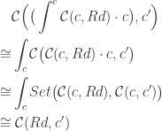
I used the fact that a hom-set from a coend is isomorphic to an end of a hom-set (continuity of hom-sets). Then I applied the definition of a tensor. Finally, I used the Yoneda lemma for contravariant functors, in which the set of natural transformations is written as an end.
![[ \mathcal{C}^{op}, Set]\big(\mathcal{C}(-, x), H \big) \cong \int_c Set \big( \mathcal{C}(c, x), H c \big) \cong H x](https://s0.wp.com/latex.php?latex=%5B+%5Cmathcal%7BC%7D%5E%7Bop%7D%2C+Set%5D%5Cbig%28%5Cmathcal%7BC%7D%28-%2C+x%29%2C+H+%5Cbig%29+%5Ccong+%5Cint_c+Set+%5Cbig%28+%5Cmathcal%7BC%7D%28c%2C+x%29%2C+H+c+%5Cbig%29+%5Ccong+H+x&bg=ffffff&fg=29303b&s=0&c=20201002)

August 22, 2020 at 3:53 am
[…] Перевод статьи Бартоша Милевски «Weighted Colimits» (исходный текст расположен по адресу — Текст оригинальной статьи). […]