The series so far:
- Hands-On with Columnstore Indexes: Part 1 Architecture
- Hands-On with Columnstore Indexes: Part 2 Best Practices and Guidelines
- Hands-On with Columnstore Indexes: Part 3 Maintenance and Additional Options
- Hands-On with Columnstore Indexes: Part 4 Query Patterns
A discussion of how columnstore indexes work is important for making the best use of them, but a practical, hands-on discussion of reality and how they are used in production environments is key to making the most of them. There are many ways that data load processes can be tweaked to dramatically improve query performance and increase scalability.
The following is a list of what I consider to be the most significant tips, tricks, and best practices for designing, loading data into, and querying columnstore indexes. As always, test all changes thoroughly before implementing them.
Columnstore indexes are generally used in conjunction with big data, and having to restructure it after-the-fact can be painfully slow. Careful design can allow a table with a columnstore index to stand on its own for a long time without the need for significant architectural changes.
Column Order is #1
Rowgroup elimination is the most significant optimization provided by a columnstore index after you account for compression. It allows large swaths of a table to be skipped when reading data, which ultimately facilitates a columnstore index growing to a massive size without the latency that eventually burdens a classic B-tree index.
Each rowgroup contains a segment for each column in the table. Metadata is stored for the segment, of which the most significant values are the row count, minimum column value, and maximum column value. For simplicity, this is akin to having MIN(), MAX(), and COUNT(*) available automatically for all segments in all rowgroups in the table.
Unlike a classic clustered B-tree index, a columnstore index has no natural concept of order. When rows are inserted into the index, they are added in the order that you insert them. If rows are inserted from ten years ago, then they will be added to the most recently available rowgroups. If rows are then inserted from today, they will get added on next. It is up to you as the architect of the table to understand what the most important column is to order by and design schema around that column.
For most OLAP tables, the time dimension will be the one that is filtered, ordered, and aggregated by. As a result, optimal rowgroup elimination requires ordering data insertion by the time dimension and maintaining that convention for the life of the columnstore index.
A basic view of segment metadata can be viewed for the date column of our columnstore index as follows:
|
1 2 3 4 5 6 7 8 9 10 11 12 13 14 15 16 17 18 19 20 21 22 23 24 25 |
SELECT tables.name AS table_name, indexes.name AS index_name, columns.name AS column_name, partitions.partition_number, column_store_segments.segment_id, column_store_segments.min_data_id, column_store_segments.max_data_id, column_store_segments.row_count FROM sys.column_store_segments INNER JOIN sys.partitions ON column_store_segments.hobt_id = partitions.hobt_id INNER JOIN sys.indexes ON indexes.index_id = partitions.index_id AND indexes.object_id = partitions.object_id INNER JOIN sys.tables ON tables.object_id = indexes.object_id INNER JOIN sys.columns ON tables.object_id = columns.object_id AND column_store_segments.column_id = columns.column_id WHERE tables.name = 'fact_order_BIG_CCI' AND columns.name = 'Order Date Key' ORDER BY tables.name, columns.name, column_store_segments.segment_id; |
The results provide segment metadata for the fact_order_BIG_CCI table and the [Order Date Key] column:
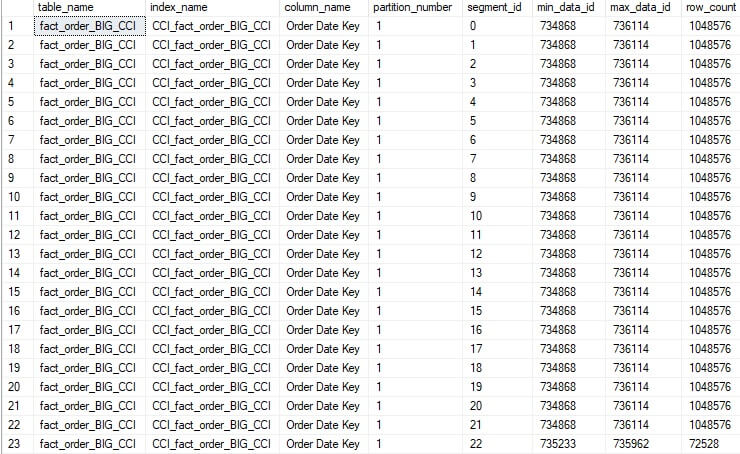
Note the columns min_data_id and max_data_id. These ID values link to dictionaries within SQL Server that store the actual minimum and maximum values. When queried, the filter values are converted to IDs and compared to the minimum and maximum values shown here. If a segment contains no values needed to satisfy a query, it is skipped. If a segment contains at least one value, then it will be included in the execution plan.
The image above highlights a BIG problem here: the minimum and maximum data ID values are the same for all but the last segment. This indicates that when the columnstore index was created, the data was not ordered by the date key. As a result, all segments will need to be read for any query against the columnstore index based on the date.
This is a common oversight, but one that is easy to correct. Note that a clustered columnstore index does not have any options that allow for order to be specified. It is up to the user to make this determination and implement it by following a process similar to this:
- Create a new table.
- Create a clustered index on the column that the table should be ordered by.
- Insert data in the order of the most significant dimension (typically date/time).
- Create the clustered columnstore index and drop the clustered B-Tree as part of its creation.
- When executing data loads, continue to insert data in the same order.
This process will create a columnstore index that is ordered solely by its most critical column and continue to maintain that order indefinitely. Consider this order to be analogous to the key columns of a classic clustered index. This may seem to be a very roundabout process, but it works effectively. Once created, the columnstore index can be inserted into using whatever key order was originally defined.
The lack of order in fact_order_BIG_CCI can be illustrated with a simple query:
|
1 2 3 4 5 6 7 |
SET STATISTICS IO ON; GO SELECT SUM([Quantity]) FROM dbo.fact_order_BIG_CCI WHERE [Order Date Key] >= '2016/01/01' AND [Order Date Key] < '2016/02/01'; |
The results return relatively quickly, but the IO details tell us something is not quite right here:

Note that 22 segments were read, and one was skipped, despite the query only looking for a single month of data. Realistically, with many years of data in this table, no more than a handful of segments should need to be read in order to satisfy such a narrow query. As long as the date values searched for appear in a limited set of rowgroups, then the rest can be automatically ignored.
With this mistake identified, let’s drop fact_order_BIG_CCI and recreate it by following this set of steps instead:
|
1 2 3 4 5 6 7 8 9 10 11 12 13 14 15 16 17 18 19 20 21 22 23 24 25 26 27 28 29 30 31 32 33 34 35 36 37 38 39 40 41 42 43 44 45 46 47 48 49 50 51 52 |
DROP TABLE dbo.fact_order_BIG_CCI; CREATE TABLE dbo.fact_order_BIG_CCI ( [Order Key] [bigint] NOT NULL, [City Key] [int] NOT NULL, [Customer Key] [int] NOT NULL, [Stock Item Key] [int] NOT NULL, [Order Date Key] [date] NOT NULL, [Picked Date Key] [date] NULL, [Salesperson Key] [int] NOT NULL, [Picker Key] [int] NULL, [WWI Order ID] [int] NOT NULL, [WWI Backorder ID] [int] NULL, [Description] [nvarchar](100) NOT NULL, [Package] [nvarchar](50) NOT NULL, [Quantity] [int] NOT NULL, [Unit Price] [decimal](18, 2) NOT NULL, [Tax Rate] [decimal](18, 3) NOT NULL, [Total Excluding Tax] [decimal](18, 2) NOT NULL, [Tax Amount] [decimal](18, 2) NOT NULL, [Total Including Tax] [decimal](18, 2) NOT NULL, [Lineage Key] [int] NOT NULL); CREATE CLUSTERED INDEX CCI_fact_order_BIG_CCI ON dbo.fact_order_BIG_CCI ([Order Date Key]); INSERT INTO dbo.fact_order_BIG_CCI SELECT [Order Key] + (250000 * ([Day Number] + ([Calendar Month Number] * 31))) AS [Order Key] ,[City Key] ,[Customer Key] ,[Stock Item Key] ,[Order Date Key] ,[Picked Date Key] ,[Salesperson Key] ,[Picker Key] ,[WWI Order ID] ,[WWI Backorder ID] ,[Description] ,[Package] ,[Quantity] ,[Unit Price] ,[Tax Rate] ,[Total Excluding Tax] ,[Tax Amount] ,[Total Including Tax] ,[Lineage Key] FROM Fact.[Order] CROSS JOIN Dimension.Date WHERE Date.Date <= '2013-04-10' ORDER BY [Order].[Order Date Key]; CREATE CLUSTERED COLUMNSTORE INDEX CCI_fact_order_BIG_CCI ON dbo.fact_order_BIG_CCI WITH (MAXDOP = 1, DROP_EXISTING = ON); |
Note that only three changes have been made to this code:
- A clustered B-tree index is created prior to any data being written to it.
- The
INSERTquery includes anORDERBYso that data is ordered by[Order Date Key]as it is added to the columnstore index. - The clustered B-tree index is swapped for the columnstore index at the end of the process.
When complete, the resulting table will contain the same data as it did at the start of this article, but physically ordered to match what makes sense for the underlying data set. This can be verified by rerunning the following query:
|
1 2 3 4 5 |
SELECT SUM([Quantity]) FROM dbo.fact_order_BIG_CCI WHERE [Order Date Key] >= '2016-01-01' AND [Order Date Key] < '2016-02-01'; |
The results show significantly improved performance:

This time, only one segment was read, and 22 were skipped. Reads are a fraction of what they were earlier. This is a significant improvement and allows us to make the most out of a columnstore index.
The takeaway of this experiment is that order matters in a columnstore index. When building a columnstore index, ensure that order is created and maintained for whatever column will be the most common filter by:
- Order the data in the initial data load. This can be accomplished by either:
- Creating a clustered B-tree index on the ordering column, populating all initial data, and then swapping it with a columnstore index.
- Create the columnstore index first, and then insert data in the correct order of the ordering column.
- Insert new data into the columnstore index using the same order every time.
Typically, the correct data order will be ascending, but do consider this detail when creating a columnstore index. If for any reason descending would make sense, be sure to design index creation and data insertion to match that order. The goal is to ensure that as few rowgroups need to be scanned as possible when executing an analytic query. When data is inserted out-of-order, the result will be that more rowgroups need to be scanned in order to fulfill that query. This may be viewed as a form of fragmentation, even though it does not fit the standard definition of index fragmentation.
Partitioning & Clustered Columnstore Indexes
Table partitioning is a natural fit for a large columnstore index. For a table that can contain row counts in the billions, it may become cumbersome to maintain all of the data in a single structure, especially if reporting needs rarely access older data.
A classic OLAP table will have both newer and older data. If common reporting queries only access a recent day, month, quarter, or year, then maintaining the older data in the same place may be unnecessary. Equally important is the fact that in an OLAP data store, older data typically does not change. If it does, it’s usually the result of software releases or other one-off operations that fall within the bounds of our world.
Table partitioning places data into multiple filegroups within a database. The filegroups can then be stored in different data files in whatever storage locations are convenient. This paradigm provides several benefits:
- Partition Elimination: Similar to rowgroup elimination, partition elimination allows partitions with unneeded data to be skipped. This can further improve performance on a large columnstore index.
- Faster Migrations: If there is a need to migrate a database to a new server or SQL Server version, then older partitions can be backed up and copied to the new data source ahead of the migration. This reduces the downtime incurred by the migration as only active data needs to be migrated during the maintenance/outage window.
Similarly, partition switching can allow for data to be moved between tables exceptionally quickly.
- Partitioned Database Maintenance: Common tasks such as backups and index maintenance can be targeted at specific partitions that contain active data. Older partitions that are static and no longer updated may be skipped.
- No Code Changes: Music to the ears of any developer: Table partitioning is a database feature that is invisible to the consumers of a table’s data. Therefore, the code needed to retrieve data before and after partitioning is added will be the same.
- Partition Column = Columnstore Order Column: The column that is used to organize the columnstore index will be the same column used in the partition function, making for an easy and consistent solution.
The fundamental steps to create a table with partitioning are as follows:
- Create filegroups for each partition based on the columnstore index ordering column.
- Create database files within each filegroup that will contain the data for each partition within the table.
- Create a partition function that determines how the data will be split based on the ordering/key column.
- Create a partition schema that binds the partition function to a set of filegroups.
- Create the table on the partition scheme defined above.
- Proceed with table population and usage as usual.
The example provided in this article can be recreated using table partitioning, though it is important to note that this is only one way to do this. There are many ways to implement partitioning, and this is not intended to be an article about partitioning, but instead introduce the idea that columnstore indexes and partitioning can be used together to continue to improve OLAP query performance.
Create New Filegroups and Files
Partitioned data can be segregated into different file groups and files. If desired, then a script similar to this would take care of the task:
|
1 2 3 4 5 6 7 8 9 10 11 12 13 14 15 16 17 18 19 20 21 22 23 24 25 26 |
ALTER DATABASE WideWorldImportersDW ADD FILEGROUP WideWorldImportersDW_2013_fg; ALTER DATABASE WideWorldImportersDW ADD FILEGROUP WideWorldImportersDW_2014_fg; ALTER DATABASE WideWorldImportersDW ADD FILEGROUP WideWorldImportersDW_2015_fg; ALTER DATABASE WideWorldImportersDW ADD FILEGROUP WideWorldImportersDW_2016_fg; ALTER DATABASE WideWorldImportersDW ADD FILEGROUP WideWorldImportersDW_2017_fg; ALTER DATABASE WideWorldImportersDW ADD FILE (NAME = WideWorldImportersDW_2013_data, FILENAME = 'C:\SQLData\WideWorldImportersDW_2013_data.ndf', SIZE = 200MB, MAXSIZE = UNLIMITED, FILEGROWTH = 1GB) TO FILEGROUP WideWorldImportersDW_2013_fg; ALTER DATABASE WideWorldImportersDW ADD FILE (NAME = WideWorldImportersDW_2014_data, FILENAME = 'C:\SQLData\WideWorldImportersDW_2014_data.ndf', SIZE = 200MB, MAXSIZE = UNLIMITED, FILEGROWTH = 1GB) TO FILEGROUP WideWorldImportersDW_2014_fg; ALTER DATABASE WideWorldImportersDW ADD FILE (NAME = WideWorldImportersDW_2015_data, FILENAME = 'C:\SQLData\WideWorldImportersDW_2015_data.ndf', SIZE = 200MB, MAXSIZE = UNLIMITED, FILEGROWTH = 1GB) TO FILEGROUP WideWorldImportersDW_2015_fg; ALTER DATABASE WideWorldImportersDW ADD FILE (NAME = WideWorldImportersDW_2016_data, FILENAME = 'C:\SQLData\WideWorldImportersDW_2016_data.ndf', SIZE = 200MB, MAXSIZE = UNLIMITED, FILEGROWTH = 1GB) TO FILEGROUP WideWorldImportersDW_2016_fg; ALTER DATABASE WideWorldImportersDW ADD FILE (NAME = WideWorldImportersDW_2017_data, FILENAME = 'C:\SQLData\WideWorldImportersDW_2017_data.ndf', SIZE = 200MB, MAXSIZE = UNLIMITED, FILEGROWTH = 1GB) TO FILEGROUP WideWorldImportersDW_2017_fg; |
The file and filegroup names are indicative of the date of the data being inserted into them. Files can be placed on different types of storage or in different locations, which can assist in growing a database over time. It can also allow for faster storage to be used for more critical data, whereas slower/cheaper storage can be used for older/less-used data.
Create a Partition Function
The partition function tells SQL Server on what boundaries to split data. For the example presented in this article, [Order Date Key], a DATE column will be used for this task:
|
1 2 3 |
CREATE PARTITION FUNCTION fact_order_BIG_CCI_years_function (DATE) AS RANGE RIGHT FOR VALUES ('2014-01-01', '2015-01-01', '2016-01-01', '2017-01-01'); |
The result of this function will be to split data into 5 ranges:
Date < 2014-01-01
Date >= 2014-01-01 & Date < 2015-01-01
Date >= 2015-01-01 & Date < 2016-01-01
Date >= 2016-01-01 & Date < 2017-01-01
Date >= 2017-01-01
Create a Partition Scheme
The partition scheme tells SQL Server where data should be physically stored, based on the function defined above. For this demo, a partition scheme such as this will give us the desired results:
|
1 2 3 4 5 |
CREATE PARTITION SCHEME fact_order_BIG_CCI_years_scheme AS PARTITION fact_order_BIG_CCI_years_function TO (WideWorldImportersDW_2013_fg, WideWorldImportersDW_2014_fg, WideWorldImportersDW_2015_fg, WideWorldImportersDW_2016_fg, WideWorldImportersDW_2017_fg); |
Each date range defined above will be assigned to a filegroup, and therefore a database file.
Create the Table
All steps performed previously to create and populate a large table with a columnstore index are identical, except for a single line within the table creation:
|
1 2 3 4 5 6 7 8 9 10 11 12 13 14 15 16 17 18 19 20 21 |
CREATE TABLE dbo.fact_order_BIG_CCI ( [Order Key] [bigint] NOT NULL, [City Key] [int] NOT NULL, [Customer Key] [int] NOT NULL, [Stock Item Key] [int] NOT NULL, [Order Date Key] [date] NOT NULL, [Picked Date Key] [date] NULL, [Salesperson Key] [int] NOT NULL, [Picker Key] [int] NULL, [WWI Order ID] [int] NOT NULL, [WWI Backorder ID] [int] NULL, [Description] [nvarchar](100) NOT NULL, [Package] [nvarchar](50) NOT NULL, [Quantity] [int] NOT NULL, [Unit Price] [decimal](18, 2) NOT NULL, [Tax Rate] [decimal](18, 3) NOT NULL, [Total Excluding Tax] [decimal](18, 2) NOT NULL, [Tax Amount] [decimal](18, 2) NOT NULL, [Total Including Tax] [decimal](18, 2) NOT NULL, [Lineage Key] [int] NOT NULL) ON fact_order_BIG_CCI_years_scheme([Order Date Key]); |
Note the final line of the query that assigns the partition scheme created above to this table. When data is written to the table, it will be written to the appropriate data file, depending on the date provided by [Order Date Key].
Testing Partitioning
The same query used to test a narrow date range can illustrate the effect that table partitioning can have on performance:
|
1 2 3 4 5 |
SELECT SUM([Quantity]) FROM dbo.fact_order_BIG_CCI WHERE [Order Date Key] >= '2016-01-01' AND [Order Date Key] < '2016-02-01'; |
The following is the IO for this query:

Instead of reading one segment and skipping 22 segments, SQL Server read one segment and skipped two. The remaining segments reside in other partitions and are automatically eliminated before reading from the table. This allows a columnstore index to have its growth split up into more manageable portions based on a time dimension. Other dimensions can be used for partitioning, though time is typically the most natural fit.
Final Notes on Partitioning
Partitioning is an optional step when implementing a columnstore index but may provide better performance and increased flexibility with regards to maintenance, software releases, and migrations.
Even if partitioning is not implemented initially, a table could be created after-the-fact and data migrated into it from the original table. Data movement such as this could be challenging in an OLTP environment, but in an OLAP database where writes are isolated, it is possible to use that period of no change to create, populate, and swap to a new table with no outage to the reporting applications that use the table.
Avoid Updates
This is worth a second mention: Avoid updates at all costs! Columnstore indexes do not treat updates efficiently. Sometimes they will perform well, especially against smaller tables, but against a large columnstore index, updates can be extremely expensive.
If data must be updated, structure it as a single delete operation followed by a single insert operation. This will take far less time to execute, cause less contention, and consume far fewer system resources.
The fact that updates can perform poorly is not well documented, so please put an extra emphasis on this fact when researching the use of columnstore indexes. If a table is being converted from a classic rowstore to a columnstore index, ensure that there are no auxiliary processes that update rows outside of the standard data load process.
Query Fewer Columns
Because data is split into segments for each column in a rowgroup, querying fewer columns means that less data needs to be retrieved in order to satisfy the query.
If a table contains 20 columns and a query performs analytics on 2 of them, then the result will be that 90% of the segments (for other columns) can be disregarded.
While a columnstore index can service SELECT * queries somewhat efficiently due to their high compression-ratio, this is not what a columnstore index is optimized to do. Like with standard clustered indexes, if a report or application does not require a column, then leave it out of the query. This will save memory, speed up reports, and make the most of columnstore indexes, which are optimized for queries against large row counts rather than large column counts.
Columnstore Compression vs. Columnstore Archive Compression
SQL Server provides an additional level of compression for columnstore indexes called Archive Compression. This shrinks the data footprint of a columnstore index further but incurs an additional CPU/duration cost to read the data.
Archive compression is meant solely for older data that is accessed infrequently and where the storage footprint is a concern. This is an important aspect of archive compression: Only use it if storage is limited, and reducing the data footprint is exceptionally beneficial. Typically, standard columnstore index compression will shrink data enough that additional savings may not be necessary.
Note that if a table is partitioned, compression can be split up such that older partitions are assigned archive compression, whereas those partitions with more frequently accessed data are assigned standard columnstore compression.
For example, the following illustrates the storage footprint of the table used in this article:
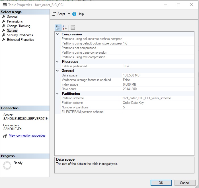
23.1 million rows are squeezed into 108MB. This is exceptional compression compared to the OLTP variant:
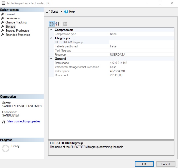
That is a huge difference! The columnstore index reduced the storage footprint from 5GB to 100MB. In a table where columns have frequently repeated values, expect to see exceptional compression ratios such as this. The less fragmented the columnstore index, the smaller the footprint becomes, as well. This columnstore index has been targeted with quite a bit of optimization throughout this article, so its fragmentation at this point in time is negligible.
For demonstration purposes, archive compression will be applied to the entire columnstore index using the following index rebuild statement:
|
1 2 3 |
ALTER INDEX CCI_fact_order_BIG_CCI ON dbo.fact_order_BIG_CCI REBUILD PARTITION = ALL WITH (DATA_COMPRESSION = COLUMNSTORE_ARCHIVE, ONLINE = ON); |
Note that the only difference is that the data compression type has been changed from columnstore to columnstore_archive. The following are the storage metrics for the table after the rebuild completes:
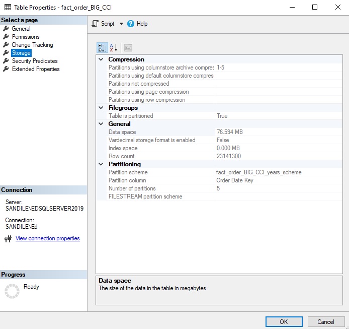
The data size has been reduced by another 25%, which is very impressive!
Archive compression is an excellent way to reduce storage footprint on data that is either:
- Accessed infrequently
- Can tolerate potentially slower execution times.
Only implement it, though, if storage is a concern and reducing data storage size is important. If using archive compression, consider combining it with table partitioning to allow for compression to be customized based on the data contained within each partition. Newer partitions can be targeted with standard columnstore compression, whereas older partitions can be targeted with archive compression.
Conclusion
The organization of data as it is loaded into a columnstore index is critical for optimizing speed. Data that is completely ordered by a common search column (typically a date or datetime) will allow for rowgroup elimination to occur naturally as the data is read. Similarly, querying fewer columns can ensure that segments are eliminated when querying across rowgroups. Lastly, implementing partitioning allows for partition elimination to occur, on top of rowgroup and segment elimination.
Combining these three features will significantly improve OLAP query performance against a columnstore index. In addition, scalability will be significantly improved as the volume of data needed to service a query will only ever be massive if there is a clear need to pull massive amounts of data. Otherwise, standard reporting needs that manage daily, weekly, monthly, quarterly, or annual analytics will not need to query any more data than is needed to return their results.

Load comments