
In the previous article, we had a chance to see how we can build Content-Based Recommendation Systems. These systems are quite easy and they consider only interaction of a single user with the items of our platform. Essentially, when we are building such a system, we describe each item using some features, i.e. we embed them in some vector space. Then we calculate similarities between each item (usually using cosine similarity). Then based on the user’s ratings and items similarities the system figures out which items should be recommended to a particular user.
We don’t do sales, but given the circumstances and the severity of the situation, we decided to change that. Don’t be fooled, this sale isn’t meant for profit and it’s most definitely not planned. This sale is here to help people who want to become better, learn new skills and be more productive than ever before. Our book offers are on a 50% sale.
This approach, however, has several shortcomings. It is limited due to the fact that it doesn’t consider other users in the system. If two users are similar, meaning that they like the same items, it makes sense to recommend them other items that one of them liked. This can not be done with content-based filtering. Another problem is that when we observe items we can “trap” users in the “recommendation bubbles“. Injecting novelty and diversity into recommendations of such system can be a challenge of its own. Finally, building this kind of system require a lot of domain knowledge, meaning we have to know a lot about every item in the platform.
Collaborative Filtering
One way to address these problems is to create a so-called Collaborative Filtering Recommendation System. Unlike Content-Based Filtering, this approach places users and items are within a common embedding space along dimensions (read – features) they have in common. For example, let’s consider that we are building a recommendation system for a platform similar to Netflix and two users of that system.


As we can see both of these users like comedy shows we could do present that like this in TensorFlow:
users_tv_shows = tf.constant([
                [10,  2,  0,  0, 0, 6],
                [0, 1,  0,  2, 10, 0]],dtype=tf.float32)
Now, we ca take the features of each show, which is just k-hot encoding of the genre:

Or in TensorFlow:
tv_shows_features = tf.constant([
                [0, 0, 1, 0, 1],
                [1, 0, 0, 0, 0],
                [1, 0, 0, 0, 0],
                [0, 1, 0, 1, 0],
                [0, 0, 1, 0, 0],
                [0, 1, 0, 0, 0]],dtype=tf.float32)
Then we can do simple dot product of these matrices and get the affinities of each user:
users_features = tf.matmul(users_tv_shows, tv_shows_features)
users_features = users_features/tf.reduce_sum(users_features, axis=1, keepdims=True)

top_users_features = tf.nn.top_k(users_features, num_feats)[1]
for i in range(num_users):
    feature_names = [features[int(index)] for index in top_users_features[i]]
    print('{}: {}'.format(users[i],feature_names))
User1: ['Comedy', 'Drama', 'Sci-Fi', 'Action', 'Cartoon']
User2: ['Comedy', 'Sci-Fi', 'Cartoon', 'Action', 'Drama']We can see that the top feature for both users is Comedy, which means they like simmilar stuff. What have we done here? Well, we not only described items in terms of the mentioned genres, but we have done the same for each user with the same terms. The meaning for a User1, for example, is that she likes Comedy 0.5 but he likes Action 0.1. Note that if we multiply users embeding matrix with the transpose item embeding matrix we will recreate the user-item interaction matrix. Now, this works well for simple examples with few users and items. However, as more items and users are added to the sytem it becomes unscalable. Also, how can we be so sure that the features that we picked are the relevant ones? What if there are some latent features, that we are unable to reckognize. So how can we pick correct features then? This brings us to the matrix factorization.
Matrix Factorization
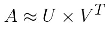
We mentioned that human-defined features for items and users might not be the best option overall. Fortunately, these embeddings can be learned from data. This means that we don’t manually assign features to the items and to the users, but we will use the user-item interaction matrix to learn the latent factors that best factorize it. As in the previous mind-exercise, this process results in a user factor embedding and item factor embedding matrixes. Technically, we are compressing a sparse user-item interaction matrix and extracting latent factors (something like PCA). That is what matrix factorization is all about, being able to factorize a matrix into two smaller matrixes using which we can reconstruct the original one:
Your content goes here. Edit or remove this text inline or in the module Content settings. You can also style every aspect of this content in the module Design settings and even apply custom CSS to this text in the module Advanced settings.

Similar to the other dimensionality reduction techniques, the number of latent features is a hyperparameter that we can change and use it for a tradeoff between more information compression and more reconstruction error. In order to make a prediction, we can do it in two ways. We can either take the dot product of a user with the item factors or the dot product of an item with the user factors. Matrix factorization helps us with one more problem. Imagine that you have thousands of users in our system and you want to calculate the similarity matrix between them. That matrix would get quite big. Matrix factorization compresses that information for us.
Algorithms
There are several good Matrix Factorization out there. So let’s explore some of the more popular ones. A couple of years back, Netflix published a $1M competition for recommendation systems. The goal was to improve the accuracy of their system based on users’ ratings. The winner used the SVD (Singular Value Decomposition) algorithm to get the best results. This algorithm is still very popular. Formally, it can be defined something like this.
Let A be an m × n matrix. The Singular Value Decomposition (SVD) of A,

where U is m × m and orthogonal, V is n × n and orthogonal, and Σ is an m × n diagonal matrix
with nonnegative diagonal entries σ1 ≥ σ2 ≥ · · · ≥ σp, p = min{m, n}, known as the singular values of A.
Another very popular algorithm is Alternating Least Squares or ALS, and their variations. Like the name suggests, it alternatively solves U holding V constant and then solves for V holding U constant and it works only for the least-squares problems. However, since it is specialized, ALS can be parallelized and it is quite fast algorythm.

One variation of it is Weighted Alternating Least Squares or WALS. The difference is in the way the missing data is treated. As we mentioned a couple of times in the previous articles, one of the biggest enemies of Recommendation Systems is sparse data. WALS adds weights for specific entries and uses those weight vector which can be linearly or exponentially scaled to normalize row and/or column frequencies.
NMF is another popular matrix factorization algorithm. It stands for non-negative matrix factorization. This technique is based on obtaining a low-rank representation of matrices with non-negative or positive elements. NMF uses an iterative procedure to modify the initial values of U and V so that the product approaches V.

Implementation
Just like in the previous article we will use MovieLens dataset for experiments, which can be downloaded from here. This dataset is a common education and practice dataset. It contains a database of movies, their genres (i.e. features), and users’ ratings of those movies. In this example, we will use only ratings.csv file (and movie.csv but just for getting titles of the movies), so let’s check out how the data looks like. Here is how it looks like when we load the data:
import numpy as np
import pandas as pd
import matplotlib.pyplot as plt

data = pd.read_csv("./data/ratings.csv")
data.head()
Data types don’t require any modifications and and there is no missing data:
data.dtypesuserId int64
movieId int64
rating float64
timestamp int64
dtype: objectdata.isnull().sum()userId 0
movieId 0
rating 0
timestamp 0
dtype: int64Distribution of ratings looks like this:
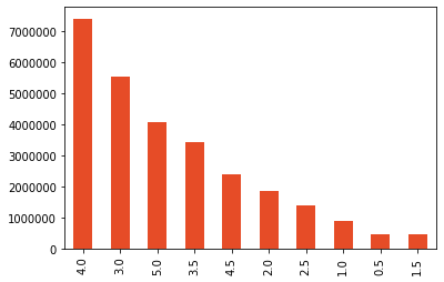
Finally, if we want more info, we can check the ratings stats:
data.rating.describe()count 2.775344e+07
mean 3.530445e+00
std 1.066353e+00
min 5.000000e-01
25% 3.000000e+00
50% 3.500000e+00
75% 4.000000e+00
max 5.000000e+00
Name: rating, dtype: float64Collaborative Filtering with Surprise
There are some great tools that can help us build recommendation systems out there. One of them is scikit’s Suprise, which stands for Simple Python RecommendatIon System Engine. It is one cool library that is going to make our lives a lot easier. The main perk for us at the moment is that we can use out of the box algorithms on MovieLense dataset. To install it you should simply run:
pip install scikit-surpriseOr using this command if you are using Anaconda:
conda install -c conda-forge scikit-surpriseNow, we are ready to implement collaborative filtering with machine learning using Surprise. First, let’s load all necessary libraries:
import numpy as np
import pandas as pd

from surprise import Reader, Dataset, SVD, BaselineOnly, NMF, accuracy
from surprise.model_selection import train_test_split
We use NumPy and Pandas for data handling and various classes and methods from Surprise. Next, we can implement DatasetBuilder class:
class DatasetBuilder():
    def __init__(self, data_location):
        reader = Reader()
        self.ratings = pd.read_csv(f"{data_location}/ratings.csv")
        self.movies = pd.read_csv(f'{data_location}/movies.csv')

        self.dataset = Dataset.load_from_df(self.ratings[['userId', 'movieId', 'rating']], reader)
        self.train_dataset, self.test_dataset = train_test_split(self.dataset, test_size=0.2)

    def get_movie_title(movie_id):
        self.movies[self.movies['movieId'] == movie_id].title
This class loads data from ratings and movie files. For the purpose of this implementation, we need only those two, with the emphasis on the ratings. Then we use Dataset class to transform data-frame with ratings into a dataset that can be used by algorithms from Surprise. Once this is done, we utilize the train_test_split method to build test and train datasets, respectively. We implement one more class AlgosGym. This class is used for training and evaluating the algorithms. Here is what it looks like:
class AlgosGym():
    def __init__(self, dataset):
        self.algos = []
        self.dataset = dataset

    def addAlgorithm(self, algo):
        self.algos.append(algo)

    def train_and_evaluate(self):
        for algo in self.algos:
            algo.fit(self.dataset.train_dataset)
            predictions = algo.test(self.dataset.test_dataset)
            rmse = accuracy.rmse(predictions)
            mae = accuracy.mae(predictions)
            fcp = accuracy.fcp(predictions)
            print('-----------')
            print(f'{algo.__class__.__name__}')
            print('-----------')
            print(f'      Metrics - RMSE: {rmse}, MAE: {mae}, FCP: {fcp}')
            print('-----------')
Essentially, using the addAlgorithm method, we can add as many algorithms as we want and when we run the train_and_evaluate method, a training procedure will be performed for all algorithms in the list. Apart from that, the number of metrics is printed out after evaluation. Let’s put all this together. First, we initialize objects for DatasetBuilder and AlgosGym as well as for SVD, NMF, and ALS. For the last one, we use BaselineOnly class. We add them all into the gym and run the train_and_evaluate method:
dataset = DatasetBuilder('./data/')
gym = AlgosGym(dataset)

svd = SVD()
gym.addAlgorithm(svd)

nmf = NMF()
gym.addAlgorithm(nmf)

bsl_options = {'method': 'als',
               'n_epochs': 5,
               'reg_u': 12,
               'reg_i': 5
               }
als = BaselineOnly(bsl_options=bsl_options)
gym.addAlgorithm(als)

gym.train_and_evaluate()
The result looks like this:
-----------
SVD
-----------
      Metrics - RMSE: 0.7940465017168126, MAE: 0.5994401838030033, FCP: 0.7331025101496759
-----------
-----------
NMF
-----------
      Metrics - RMSE: 0.87889005723462, MAE: 0.6708987729904538, FCP: 0.6815580327751358
-----------
-----------
BaselineOnly
-----------
      Metrics - RMSE: 0.8688777191828219, MAE: 0.6646682407762424, FCP: 0.6855766028894256
-----------
Now, these metrics are nice indications, however, they can be a wrong path. This means that we need additionally to observe what the user liked in order to determine which algorithm performed the best.
Conclusion
In this article, we learned how we can build a simple collaborative filtering recommendation system using machine learning. We used the Surprise library and algorithms with matrix factorization. Also, we learned other algorithms that could be used for this purpose as well. Thank you for reading!

Nikola M. Zivkovic
CAIO at Rubik's Code
Nikola M. Zivkovic a CAIO at Rubik’s Code and the author of book “Deep Learning for Programmers“. He is loves knowledge sharing, and he is experienced speaker. You can find him speaking at meetups, conferences and as a guest lecturer at the University of Novi Sad.
Rubik’s Code is a boutique data science and software service company with more than 10 years of experience in Machine Learning, Artificial Intelligence & Software development. Check out the services we provide.


Trackbacks/Pingbacks