MotionPlanner
The goal of this project will be to have a functional motion planning stack that can avoid both static and dynamic obstacles while tracking the center line of a lane, while also handling stop signs. To accomplish this, we will have to implement behavioral planning logic, as well as static collision checking, path selection, and velocity profile generation.
General Overview and some key concepts
Implementing the Motion Planner
In this project, we will be editing the "behavioural_planner.py", "collision_checker.py", "local_planner.py", "path_optimizer.py", and "velocity_planner.py" class files (found inside the "PythonClient\Course4FinalProject" (for Windows) or "PythonClient/Course4FinalProject" (for Ubuntu) folder). This is where we will implement our motion planner. There are 5 main aspects of the planner you will need to implement, behaviour planning logic, path generation, static collision checking, path selection, and velocity profile generation
Solution Approach
Path Generation

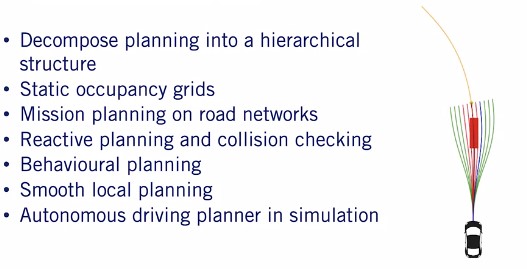
We had given you all of the required code to optimize a spiral to a given point. So all we needed to add was to extract the goal points from the way points sequence you were given. We did this by iterating through the way points and finding the closest one to the ego vehicle, and then progressing through way points until we arrived at a way point that was at least a look ahead distance away from us. The look ahead distance represents how far ahead of the vehicle we are planning during any cycle. Once this goal point is selected, we laterally offset additional goal points from the selected way point to generate a goal state set. We do this to give the car multiple options to select from, which will allow it to avoid obstacles. The lateral spacing is 90 degrees rotated away from the heading of the road at the target way point. This ensures that our planned path set conforms to the structure of the road. We then have to rotate and translate these points from the global frame to the ego vehicles frame, such that the ego vehicle is at the origin with zero heading. Once this is done, we can pass these goal points to the spiral optimizer which will then compute the path that we can use in our future planning steps.
Collision Avoidance

Once we have our path set, the next step to perform is collision checking and path selection. To compute the best feasible and collision-free path for our ego vehicle to follow. The way we performed collision checking was to use the circle based method we introduced in Module Four. In particular, we overlaid circles on top of the vehicle location at each point along the path. This generates a set of circles which gives us a conservative approximation of the ego vehicle swath. We then checked if each of the obstacle points was located within any of the circles along the path. If any of the points did fall within the circles, then this path was labeled as having a collision. We then repeated this process for each of the paths removing all of those that collided with obstacles from future consideration. Once our collision check was complete, we then selected the collision-free path whose end-point was closest to the line center line as our best path. We select this because it allows us to track the global way points along the center of the lane even if we had to veer off course temporarily due to an obstacle along our path. This choice does lead us to cut as close as possible to obstacles. So we had to be careful to ensure our collision checks were conservative with some buffer.
Velocity Profile Generation

Once we have a suitable path selected, we need to generate a velocity profile for it. We are given a reference velocity depending on the behavior we are trying to execute. If we are decelerating to a stop or staying stopped, our target velocity should be zero. Otherwise, it should be the speed limit. However, we need to take leading vehicles into consideration. Because if a leading vehicle is moving more slowly than us we may hit it. To handle this, we set our target velocity to be the minimum of the reference velocity, and the lead vehicle speed. We also need to make sure that we reach the lead vehicle speed by the time we reach the lead vehicles original location. Otherwise we risk a collision. From this information, we can now construct a ramp trajectory from our current velocity, to the target velocity along our path. If there is a lead vehicle, the end-point of the ramp profile will be the lead vehicles position less a time gap buffer. Otherwise the end-point of the ramp profile will be the end of the path.
Behaviour Planning

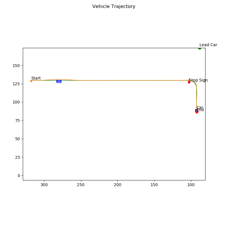
Finally, we must implement the behavioral planner for our ego vehicle. The only regulatory element we will face in this project is a stop sign, so that will be the focus of the behavioral planner. To handle it, our behavioral planner will have three states. A nominal lane following state, a decelerate to stop state, and a stay stop state. During the course of normal driving we will stay in the lane following state. Once the endpoint of our planned path crosses the stop line of a stop sign, we then switch from driving normally to decelerating to a stop at the stop point defined by that stopline. To do this, we must transition to the decelerate to stop state, and ensure our planned length provides sufficient time to decelerate comfortably. Once we've stopped we transition to the stay stopped state to make sure the car is at a complete stop at the stop sign for a fixed period of time. In this case, we choose two seconds. Once that is done, we then transition back to the lane following state, and continue with nominal driving. This completes the state machine transition cycle, and allows us to handle the presence of a stop sign along our path.
Final Results


Installing and Running
- Download this repository file and unpack into the subfolder folder "PythonClient" inside the "CarlaSimulator" (root) folder.
Running the CARLA simulator
- In one terminal, start the CARLA simulator at a 30hz fixed time-step:
Ubuntu:
./CarlaUE4.sh /Game/Maps/Course4 -windowed -carla-server -benchmark -fps=30
Windows:
CarlaUE4.exe /Game/Maps/Course4 -windowed -carla-server -benchmark -fps=30
- Note that both the ResX=<pixel_width> and ResY=<pixel_height> arguments can used to create a fixed size window, if you find the simulation to run too slow.
Running the Python client (and controller)
-
In another terminal, change the directory to go into the "Course4FinalProject" folder, under the "PythonClient" folder.
-
Run your controller, execute the following command while CARLA is open:
Ubuntu (use alternative python commands if the command below does not work, as described in the CARLA install guide):
python3 module_7.py
Windows (use alternative python commands if the command below does not work, as described in the CARLA install guide):
python module_7.py
Changing the live plotter refresh rate
-
If the simulation runs slowly, you can try increasing the period at which the live plotter refreshes the plots, or disabling the live plotting altogether. Disabling the live plotting or changing its refresh rate does not affect the plot outputs at the end of the simulation.
-
To do this, edit the options.cfg file found in the "Course1FinalProject" folder for the relevant parameters. The following table below explains each option:
| Parameter | Description | Value |
|---|---|---|
| live_plotting | Enable or disable live plotting. | true/false |
| live_plotting_period | Period (in seconds) which the live plot will refresh on screen. | seconds |
Final Notes:
- This is the final assignment project from Motion Planning for Self-Driving Cars course of Self-Driving Cars Specialization by University of Toronto.


