The following problems appeared as assignments in the edX course Analytics for Computing (by Gatech). The descriptions are taken from the assignments.
1. Association rule mining
First we shall implement the basic pairwise association rule mining algorithm.
Problem definition
Let’s say we have a fragment of text in some language. We wish to know whether there are association rules among the letters that appear in a word. In this problem:
- Words are “receipts”
- Letters within a word are “items”
We want to know whether there are association rules of the form, a⟹ b , where a and b are letters, for a given language (by calculating for each rule its confidence, conf (a ⟹ b), which is an estimate of the conditional probability of b given a, or Pr[b|a].
Sample text input
Let’s carry out this analysis on a “dummy” text fragment, which graphic designers refer to as the lorem ipsum:
latin_text= """
Sed ut perspiciatis, unde omnis iste natus error sit voluptatem accusantium doloremque laudantium, totam
rem aperiam eaque ipsa, quae ab illo inventore veritatis et quasi architecto beatae vitae dicta
sunt, explicabo. Nemo enim ipsam voluptatem, quia voluptas sit, aspernatur aut odit aut fugit, sed
quia consequuntur magni dolores eos, qui ratione voluptatem sequi nesciunt, neque porro quisquam est,
qui dolorem ipsum, quia dolor sit amet consectetur adipisci[ng] velit, sed quia non numquam [do] eius
modi tempora inci[di]dunt, ut labore et dolore magnam aliquam quaerat voluptatem. Ut enim ad minima
veniam, quis nostrum exercitationem ullam corporis suscipit laboriosam, nisi ut aliquid ex ea commodi
consequatur? Quis autem vel eum iure reprehenderit, qui in ea voluptate velit esse, quam nihil molestiae
consequatur, vel illum, qui dolorem eum fugiat, quo voluptas nulla pariatur?

At vero eos et accusamus et iusto odio dignissimos ducimus, qui blanditiis praesentium voluptatum
deleniti atque corrupti, quos dolores et quas molestias excepturi sint, obcaecati cupiditate non
provident, similique sunt in culpa, qui officia deserunt mollitia animi, id est laborum et dolorum
fuga. Et harum quidem rerum facilis est et expedita distinctio. Nam libero tempore, cum soluta nobis est
eligendi optio, cumque nihil impedit, quo minus id, quod maxime placeat, facere possimus, omnis voluptas
assumenda est, omnis dolor repellendus. Temporibus autem quibusdam et aut officiis debitis aut rerum
necessitatibus saepe eveniet, ut et voluptates repudiandae sint et molestiae non recusandae. Itaque
earum rerum hic tenetur a sapiente delectus, ut aut reiciendis voluptatibus maiores alias consequatur
aut perferendis doloribus asperiores repellat.
"""
Data cleaning
Like most data in the real world, this dataset is noisy. It has both uppercase and lowercase letters, words have repeated letters, and there are all sorts of non-alphabetic characters. For our analysis, we should keep all the letters and spaces (so we can identify distinct words), but we should ignore case and ignore repetition within a word.
For example, the eighth word of this text is “error.” As an itemset, it consists of the three unique letters, {e,o,r}. That is, to treat the word as a set, meaning we only keep the unique letters. This itemset has six possible itempairs: {e,o}, {e,r}, and {o,r}.
- We need to start by “cleaning up” (normalizing) the input, with all characters converted to lowercase and all non-alphabetic, non-space characters removed.
- Next, we need to convert each word into an itemset like the following examples:
consequatur –> {‘a’, ‘e’, ‘c’, ‘s’, ‘n’, ‘o’, ‘u’, ‘t’, ‘q’, ‘r’}
voluptatem –> {‘l’, ‘a’, ‘e’, ‘o’, ‘p’, ‘u’, ‘m’, ‘t’, ‘v’}
Implementing the basic algorithm
The followed algorithm is implemented:
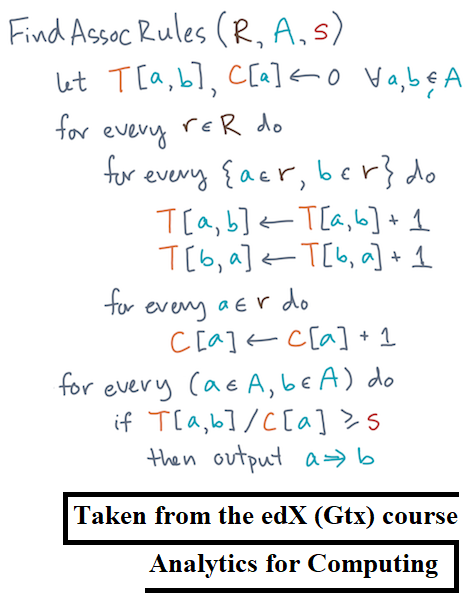
First all item-pairs within an itemset are enumerated and a table that tracks the counts of those item-pairs is updated in-place.
- Now, given tables of item-paircounts and individual item counts, as well as a confidence threshold, the rules that meet the threshold are returned.
- The returned rules should be in the form of a dictionary whose key is the tuple, (a,b) corresponding to the rule a⇒ b, and whose value is the confidence of the rule, conf(a ⇒ b).
- The following functions were implemented to compute the association rules.
from collections import defaultdict
from itertools import combinations

def update_pair_counts (pair_counts, itemset):
    """
    Updates a dictionary of pair counts for all pairs of items
    in a given itemset.
    """
    assert type (pair_counts) is defaultdict

    for item in list(combinations(itemset, 2)):
        pair_counts[item] += 1
        pair_counts[item[::-1]] += 1
    return pair_counts
def update_item_counts(item_counts, itemset):

    for item in itemset:
        item_counts[item] += 1
    return item_counts
def filter_rules_by_conf (pair_counts, item_counts, threshold):
    rules = {} # (item_a, item_b) -> conf (item_a => item_b)

    for (item_a, item_b) in pair_counts:
        conf = pair_counts[(item_a, item_b)] / float(item_counts[item_a])
        if conf >= threshold:
            rules[(item_a, item_b)] = conf

    return rules
def find_assoc_rules(receipts, threshold):

    pair_counts = defaultdict(int)
    item_counts = defaultdict(int)
    for receipt in receipts:
        update_pair_counts(pair_counts, receipt)
        update_item_counts(item_counts, receipt)
    return filter_rules_by_conf(pair_counts, item_counts, threshold)
- For the Latin string,
latin_text, the functionfind_assoc_rules()was used to compute the rules whose confidence is at least 0.75, with the following rules obtained as result.
conf(q => u) = 1.000
conf(x => e) = 1.000
conf(x => i) = 0.833
conf(h => i) = 0.833
conf(v => t) = 0.818
conf(r => e) = 0.800
conf(v => e) = 0.773
conf(f => i) = 0.750
conf(b => i) = 0.750
conf(g => i) = 0.750
- Now, let’s look at rules common to the above Latin textandEnglish text obtained by a translation of the lorem ipsum text, as shown below:
english_text = """
But I must explain to you how all this mistaken idea of denouncing of a pleasure and praising pain was
born and I will give you a complete account of the system, and expound the actual teachings of the great
explorer of the truth, the master-builder of human happiness. No one rejects, dislikes, or avoids
pleasure itself, because it is pleasure, but because those who do not know how to pursue pleasure
rationally encounter consequences that are extremely painful. Nor again is there anyone who loves or
pursues or desires to obtain pain of itself, because it is pain, but occasionally circumstances occur in
which toil and pain can procure him some great pleasure. To take a trivial example, which of us
ever undertakes laborious physical exercise, except to obtain some advantage from it? But who has any
right to find fault with a man who chooses to enjoy a pleasure that has no annoying consequences, or
one who avoids a pain that produces no resultant pleasure?

On the other hand, we denounce with righteous indignation and dislike men who are so beguiled and
demoralized by the charms of pleasure of the moment, so blinded by desire, that they cannot foresee the
pain and trouble that are bound to ensue; and equal blame belongs to those who fail in their duty
through weakness of will, which is the same as saying through shrinking from toil and pain. These
cases are perfectly simple and easy to distinguish. In a free hour, when our power of choice is
untrammeled and when nothing prevents our being able to do what we like best, every pleasure is to
be welcomed and every pain avoided. But in certain circumstances and owing to the claims of duty or
the obligations of business it will frequently occur that pleasures have to be repudiated and
annoyances accepted. The wise man therefore always holds in these matters to this principle of
selection: he rejects pleasures to secure other greater pleasures, or else he endures pains to
avoid worse pains.
"""
- Again, for the English string,
english_text, the functionfind_assoc_rules()was used to compute the rules whose confidence is at least 0.75, with the following rules obtained as result.
conf(z => a) = 1.000
conf(j => e) = 1.000
conf(z => o) = 1.000
conf(x => e) = 1.000
conf(q => e) = 1.000
conf(q => u) = 1.000
conf(z => m) = 1.000
conf(z => r) = 1.000
conf(z => l) = 1.000
conf(z => e) = 1.000
conf(z => d) = 1.000
conf(z => i) = 1.000
conf(k => e) = 0.778
conf(q => n) = 0.750
- Let’s consider any rules with a confidence of at least 0.75 to be a “high-confidence rule“. The
common_high_conf_rulesare all the high-confidence rules appearing in both the Latin text and the English text. The rules shown below are all such rules:High-confidence rules common to _lorem ipsum_ in Latin and English:
q => u
x => e
- The following table and the figure show the high confidence rules for the latin and the english texts.
index rule confidence 0 z=> o 1.000000 English 1 z=> l 1.000000 English 2 z=> m 1.000000 English 3 q=> u 1.000000 English 4 q=> e 1.000000 English 5 x=> e 1.000000 English 6 z=> e 1.000000 English 7 j=> e 1.000000 English 8 z=> a 1.000000 English 9 z=> d 1.000000 English 10 q=> u 1.000000 Latin 11 z=> i 1.000000 English 12 x=> e 1.000000 Latin 13 z=> r 1.000000 English 14 x=> i 0.833333 Latin 15 h=> i 0.833333 Latin 16 v=> t 0.818182 Latin 17 r=> e 0.800000 Latin 18 k=> e 0.777778 English 19 v=> e 0.772727 Latin 20 g=> i 0.750000 Latin 21 q=> n 0.750000 English 22 f=> i 0.750000 Latin 23 b=> i 0.750000 Latin 
Putting it all together: Actual baskets!
Let’s take a look at some real data from this link. First few lines of the transaction data is shown below:
citrus fruit,semi-finished bread,margarine,ready soups
tropical fruit,yogurt,coffee
whole milk
pip fruit,yogurt,cream cheese ,meat spreads
other vegetables,whole milk,condensed milk,long life bakery product
whole milk,butter,yogurt,rice,abrasive cleaner
rolls/buns
other vegetables,UHT-milk,rolls/buns,bottled beer,liquor (appetizer)
pot plants
whole milk,cereals
tropical fruit,other vegetables,white bread,bottled water,chocolate
citrus fruit,tropical fruit,whole milk,butter,curd,yogurt,flour,bottled water,dishes
beef
frankfurter,rolls/buns,soda
chicken,tropical fruit
butter,sugar,fruit/vegetable juice,newspapers
fruit/vegetable juice
packaged fruit/vegetables
chocolate
specialty bar
other vegetables
butter milk,pastry
whole milk
tropical fruit,cream cheese ,processed cheese,detergent,newspapers
tropical fruit,root vegetables,other vegetables,frozen dessert,rolls/buns,flour,sweet spreads,salty snack,waffles,candy,bathroom cleaner
bottled water,canned beer
yogurt
sausage,rolls/buns,soda,chocolate
other vegetables
brown bread,soda,fruit/vegetable juice,canned beer,newspapers,shopping bags
yogurt,beverages,bottled water,specialty bar
- Our task is to mine this dataset for pairwise association rules to produce a final dictionary,
basket_rules, that meet these conditions:
- The keys are pairs (a,b), where a and b are item names.
- The values are the corresponding confidence scores, conf(a ⇒ b).
- Only include rules a ⇒ b where item a occurs at least
MIN_COUNTtimes and conf(a ⇒ b) is at leastTHRESHOLD.
The result is shown below:
Found 19 rules whose confidence exceeds 0.5.
Here they are:conf(honey => whole milk) = 0.733
conf(frozen fruits => other vegetables) = 0.667
conf(cereals => whole milk) = 0.643
conf(rice => whole milk) = 0.613
conf(rubbing alcohol => whole milk) = 0.600
conf(cocoa drinks => whole milk) = 0.591
conf(pudding powder => whole milk) = 0.565
conf(jam => whole milk) = 0.547
conf(cream => sausage) = 0.538
conf(cream => other vegetables) = 0.538
conf(baking powder => whole milk) = 0.523
conf(tidbits => rolls/buns) = 0.522
conf(rice => other vegetables) = 0.520
conf(cooking chocolate => whole milk) = 0.520
conf(frozen fruits => whipped/sour cream) = 0.500
conf(specialty cheese => other vegetables) = 0.500
conf(ready soups => rolls/buns) = 0.500
conf(rubbing alcohol => butter) = 0.500
conf(rubbing alcohol => citrus fruit) = 0.500
2. Simple string processing with Regex
Phone numbers
- Write a function to parse US phone numbers written in the canonical “(404) 555-1212” format, i.e., a three-digit area code enclosed in parentheses followed by a seven-digit local number in three-hyphen-four digit format.
- It should also ignore all leading and trailing spaces, as well as any spaces that appear between the area code and local numbers.
- However, it should not accept any spaces in the area code (e.g., in ‘(404)’) nor should it in the local number.
- It should return a triple of strings,
(area_code, first_three, last_four).
- If the input is not a valid phone number, it should raise a
ValueError.
import re
def parse_phone(s):
    pattern = re.compile("\s*\((\d{3})\)\s*(\d{3})-(\d{4})\s*")
    m = pattern.match(s)
    if not m:
        raise ValueError('not a valid phone number!')
    return m.groups()

#print(parse_phone1('(404) 201-2121'))
#print(parse_phone1('404-201-2121'))
- Implement an enhanced phone number parser that can handle any of these patterns.
- (404) 555-1212
- (404) 5551212
- 404-555-1212
- 404-5551212
- 404555-1212
- 4045551212
- As before, it should not be sensitive to leading or trailing spaces. Also, for the patterns in which the area code is enclosed in parentheses, it should not be sensitive to the number of spaces separating the area code from the remainder of the number.
The following function implements the enhanced regex parser.
import re
def parse_phone2 (s):
    pattern = re.compile("\s*\((\d{3})\)\s*(\d{3})-?(\d{4})\s*")
    m = pattern.match(s)
    if not m:
        pattern2 = re.compile("\s*(\d{3})-?(\d{3})-?(\d{4})\s*")
        m = pattern2.match(s)
        if not m:
            raise ValueError('not a valid phone number!')
    return m.groups()
3. Tidy data and the Pandas
“Tidying data,” is all about cleaning up tabular data for analysis purposes.
Definition: Tidy datasets. More specifically, Wickham defines a tidy data set as one that can be organized into a 2-D table such that
- each column represents a variable;
- each row represents an observation;
- each entry of the table represents a single value, which may come from either categorical (discrete) or continuous spaces.
Definition: Tibbles. if a table is tidy, we will call it a tidy table, or tibble, for short.
Apply functions to data frames
Given the following pandas DataFrame (first few rows are shown in the next table),compute the prevalence, which is the ratio of cases to the population, using the apply() function, without modifying the original DataFrame.
| country | year | cases | population | |
|---|---|---|---|---|
| 0 | Afghanistan | ’99 | 745 | 19987071 |
| 1 | Brazil | ’99 | 37737 | 172006362 |
| 2 | China | ’99 | 212258 | 1272915272 |
| 3 | Afghanistan | ’00 | 2666 | 20595360 |
| 4 | Brazil | ’00 | 80488 | 174504898 |
| 5 | China | ’00 | 213766 | 1280428583 |
The next function does exactly the same thing.
def calc_prevalence(G):
    assert 'cases' in G.columns and 'population' in G.columns
    H = G.copy()
    H['prevalence'] = H.apply(lambda row: row['cases'] / row['population'], axis=1)
    return H
Tibbles and Bits
Now let’s start creating and manipulating tibbles.
Write a function, canonicalize_tibble(X), that, given a tibble X, returns a new copy Y of X in canonical order. We say Y is in canonical order if it has the following properties.
- The variables appear in sorted order by name, ascending from left to right.
- The rows appear in lexicographically sorted order by variable, ascending from top to bottom.
- The row labels (
Y.index) go from 0 ton-1, wherenis the number of observations.
The following code exactly does the same:
def canonicalize_tibble(X):
    # Enforce Property 1:
    var_names = sorted(X.columns)
    Y = X[var_names].copy()
    Y = Y.sort_values(by=var_names, ascending=True)
    Y.reset_index(drop=True, inplace=True)
    return Y
Basic tidying transformations: Implementing Melting and Casting
Given a data set and a target set of variables, there are at least two common issues that require tidying.
Melting
First, values often appear as columns. Table 4a is an example. To tidy up, we want to turn columns into rows:

Because this operation takes columns into rows, making a “fat” table more tall and skinny, it is sometimes called melting.
To melt the table, we need to do the following.
- Extract the column values into a new variable. In this case, columns
"1999"and"2000"oftable4need to become the values of the variable,"year". - Convert the values associated with the column values into a new variable as well. In this case, the values formerly in columns
"1999"and"2000"become the values of the"cases"variable.
In the context of a melt, let’s also refer to "year" as the new key variable and
"cases" as the new value variable.
Implement the melt operation as a function,
def melt(df, col_vals, key, value):
        ...
It should take the following arguments:
df: the input data frame, e.g.,table4in the example above;col_vals: a list of the column names that will serve as values;key: name of the new variable, e.g.,yearin the example above;value: name of the column to hold the values.
The next function implements the melt operation:
def melt(df, col_vals, key, value):
    assert type(df) is pd.DataFrame
    df2 = pd.DataFrame()
    for col in col_vals:
        df1 = pd.DataFrame(df[col].tolist(), columns=[value]) #, index=df.country)
        df1[key] = col
        other_cols = list(set(df.columns.tolist()) - set(col_vals))
        for col1 in other_cols:
            df1[col1] = df[col1]
        df2 = df2.append(df1, ignore_index=True)
    df2 = df2[other_cols + [key, value]]
    return df2
with the following output
| country | year | population | |
|---|---|---|---|
| 0 | Afghanistan | 1999 | 19987071 |
| 1 | Brazil | 1999 | 172006362 |
| 2 | China | 1999 | 1272915272 |
| 3 | Afghanistan | 2000 | 20595360 |
| 4 | Brazil | 2000 | 174504898 |
| 5 | China | 2000 | 1280428583 |
Casting
The second most common issue is that an observation might be split across multiple rows. Table 2 is an example. To tidy up, we want to merge rows:
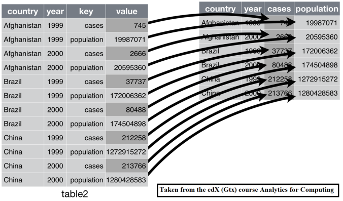
Because this operation is the moral opposite of melting, and “rebuilds” observations from parts, it is sometimes called casting.
Melting and casting are Wickham’s terms from his original paper on tidying data. In his more recent writing, on which this tutorial is based, he refers to the same operation as gathering. Again, this term comes from Wickham’s original paper, whereas his more recent summaries use the term spreading.
The signature of a cast is similar to that of melt. However, we only need to know the key, which is column of the input table containing new variable names, and the value, which is the column containing corresponding values.
Implement a function to cast a data frame into a tibble, given a key column containing new variable names and a value column containing the corresponding cells.
Observe that we are asking your cast() to accept an optional parameter, join_how, that may take the values 'outer' or 'inner' (with 'outer' as the default).
The following function implements the casting operation:
def cast(df, key, value, join_how='outer'):
    """Casts the input data frame into a tibble,
    given the key column and value column.
    """
    assert type(df) is pd.DataFrame
    assert key in df.columns and value in df.columns
    assert join_how in ['outer', 'inner']

    fixed_vars = df.columns.difference([key, value])
    tibble = pd.DataFrame(columns=fixed_vars) # empty frame

    fixed_vars = fixed_vars.tolist()
    #tibble[fixed_vars] = df[fixed_vars]
    cols = []
    for k,df1 in df.groupby(df[key]):
        #tibble = pd.concat([tibble.reset_index(drop=True), df1[value]], axis=1)
        #print(df1[fixed_vars+[value]].head())
        tibble = tibble.merge(df1[fixed_vars+[value]], on=fixed_vars, how=join_how)
        cols.append(str(k)) #list(set(df1[key]))[0])
    tibble.columns = fixed_vars + cols

    return tibble
with the following output:
Separating variables
Consider the following table.
| country | year | rate | |
|---|---|---|---|
| 0 | Afghanistan | 1999 | 745/19987071 |
| 1 | Afghanistan | 2000 | 2666/20595360 |
| 2 | Brazil | 1999 | 37737/172006362 |
| 3 | Brazil | 2000 | 80488/174504898 |
| 4 | China | 1999 | 212258/1272915272 |
| 5 | China | 2000 | 213766/1280428583 |
In this table, the rate variable combines what had previously been the cases
andpopulation data. This example is an instance in which we might want to separate a column into two variables.
Write a function that takes a data frame (df) and separates an existing column (key) into new variables (given by the list of new variable names, into). How will the separation happen? The caller should provide a function, splitter(x), that given a value returns a list containing the components.
The following code implements the function:
import re

def default_splitter(text):
    """Searches the given spring for all integer and floating-point
    values, returning them as a list _of strings_.

    E.g., the call

      default_splitter('Give me $10.52 in exchange for 91 kitten stickers.')

    will return ['10.52', '91'].
    """
    #fields = re.findall('(\d+\.?\d+)', text)
    fields = list(re.match('(\d+)/(\d+)', text).groups())
    return fields

def separate(df, key, into, splitter=default_splitter):
    """Given a data frame, separates one of its columns, the key,
    into new variables.
    """
    assert type(df) is pd.DataFrame
    assert key in df.columns
    return (df.merge(df[key].apply(lambda s: pd.Series({into[i]:splitter(s)[i] for i in range(len(into))})),
    left_index=True, right_index=True)).drop(key, axis=1)
with the following output:

Nice explanations. Thanks.
LikeLike