The Generative Adversarial Network, or GAN, is an architecture for training deep convolutional models for generating synthetic images.
Although remarkably effective, the default GAN provides no control over the types of images that are generated. The Information Maximizing GAN, or InfoGAN for short, is an extension to the GAN architecture that introduces control variables that are automatically learned by the architecture and allow control over the generated image, such as style, thickness, and type in the case of generating images of handwritten digits.
In this tutorial, you will discover how to implement an Information Maximizing Generative Adversarial Network model from scratch.
After completing this tutorial, you will know:
The InfoGAN is motivated by the desire to disentangle and control the properties in generated images.
The InfoGAN involves the addition of control variables to generate an auxiliary model that predicts the control variables, trained via mutual information loss function.
How to develop and train an InfoGAN model from scratch and use the control variables to control which digit is generated by the model.
Update Oct/2019: Fixed typo in explanation of mutual information loss.
Update Jan/2021: Updated so layer freezing works with batch norm.
How to Develop an Information Maximizing Generative Adversarial Network (InfoGAN) in Keras Photo by Irol Trasmonte, some rights reserved.
Tutorial Overview
This tutorial is divided into four parts; they are:
What Is the Information Maximizing GAN
How to Implement the InfoGAN Loss Function
How to Develop an InfoGAN for MNIST
How to Use Control Codes With a Trained InfoGAN Model
What Is the Information Maximizing GAN
The Generative Adversarial Network, or GAN for short, is an architecture for training a generative model, such as a model for generating synthetic images.
It involves the simultaneous training of the generator model for generating images with a discriminator model that learns to classify images as either real (from the training dataset) or fake (generated). The two models compete in a zero-sum game such that convergence of the training process involves finding a balance between the generator’s skill in generating convincing images and the discriminator’s in being able to detect them.
The generator model takes as input a random point from a latent space, typically 50 to 100 random Gaussian variables. The generator applies a unique meaning to the points in the latent space via training and maps points to specific output synthetic images. This means that although the latent space is structured by the generator model, there is no control over the generated image.
The GAN formulation uses a simple factored continuous input noise vector z, while imposing no restrictions on the manner in which the generator may use this noise. As a result, it is possible that the noise will be used by the generator in a highly entangled way, causing the individual dimensions of z to not correspond to semantic features of the data.
The latent space can be explored and generated images compared in an attempt to understand the mapping that the generator model has learned. Alternatively, the generation process can be conditioned, such as via a class label, so that images of a specific type can be created on demand. This is the basis for the Conditional Generative Adversarial Network, CGAN or cGAN for short.
Another approach is to provide control variables as input to the generator, along with the point in latent space (noise). The generator can be trained to use the control variables to influence specific properties of the generated images. This is the approach taken with the Information Maximizing Generative Adversarial Network, or InfoGAN for short.
InfoGAN, an information-theoretic extension to the Generative Adversarial Network that is able to learn disentangled representations in a completely unsupervised manner.
The structured mapping learned by the generator during the training process is somewhat random. Although the generator model learns to spatially separate properties of generated images in the latent space, there is no control. The properties are entangled. The InfoGAN is motivated by the desire to disentangle the properties of generated images.
For example, in the case of faces, the properties of generating a face can be disentangled and controlled, such as the shape of the face, hair color, hairstyle, and so on.
For example, for a dataset of faces, a useful disentangled representation may allocate a separate set of dimensions for each of the following attributes: facial expression, eye color, hairstyle, presence or absence of eyeglasses, and the identity of the corresponding person.
Control variables are provided along with the noise as input to the generator and the model is trained via a mutual information loss function.
… we present a simple modification to the generative adversarial network objective that encourages it to learn interpretable and meaningful representations. We do so by maximizing the mutual information between a fixed small subset of the GAN’s noise variables and the observations, which turns out to be relatively straightforward.
Mutual information refers to the amount of information learned about one variable given another variable. In this case, we are interested in the information about the control variables given the image generated using noise and the control variables.
In information theory, mutual information between X and Y , I(X; Y ), measures the “amount of information” learned from knowledge of random variable Y about the other random variable X.
The Mutual Information (MI) is calculated as the conditional entropy of the control variables (c) given the image (created by the generator (G) from the noise (z) and the control variable (c)) subtracted from the marginal entropy of the control variables (c); for example:
MI = Entropy(c) – Entropy(c ; G(z,c))
Calculating the true mutual information, in practice, is often intractable, although simplifications are adopted in the paper, referred to as Variational Information Maximization, and the entropy for the control codes is kept constant. For more on mutual information, see the tutorial:
Training the generator via mutual information is achieved through the use of a new model, referred to as Q or the auxiliary model. The new model shares all of the same weights as the discriminator model for interpreting an input image, but unlike the discriminator model that predicts whether the image is real or fake, the auxiliary model predicts the control codes that were used to generate the image.
Both models are used to update the generator model, first to improve the likelihood of generating images that fool the discriminator model, and second to improve the mutual information between the control codes used to generate an image and the auxiliary model’s prediction of the control codes.
The result is that the generator model is regularized via mutual information loss such that the control codes capture salient properties of the generated images and, in turn, can be used to control the image generation process.
… mutual information can be utilized whenever we are interested in learning a parametrized mapping from a given input X to a higher level representation Y which preserves information about the original input. […] show that the task of maximizing mutual information is essentially equivalent to training an autoencoder to minimize reconstruction error.
Take my free 7-day email crash course now (with sample code).
Click to sign-up and also get a free PDF Ebook version of the course.
How to Implement the InfoGAN Loss Function
The InfoGAN is reasonably straightforward to implement once you are familiar with the inputs and outputs of the model.
The only stumbling block might be the mutual information loss function, especially if you don’t have a strong math background, like most developers.
There are two main types of control variables used with the InfoGan: categorical and continuous, and continuous variables may have different data distributions, which impact how the mutual loss is calculated. The mutual loss can be calculated and summed across all control variables based on the variable type, and this is the approach used in the official InfoGAN implementation released by OpenAI for TensorFlow.
In Keras, it might be easier to simplify the control variables to categorical and either Gaussian or Uniform continuous variables and have separate outputs on the auxiliary model for each control variable type. This is so that a different loss function can be used, greatly simplifying the implementation.
See the papers and posts in the further reading section for more background on the recommendations in this section.
Categorical Control Variables
The categorical variable may be used to control the type or class of the generated image.
This is implemented as a one hot encoded vector. That is, if the class has 10 values, then the control code would be one class, e.g. 6, and the categorical control vector input to the generator model would be a 10 element vector of all zero values with a one value for class 6, for example, [0, 0, 0, 0, 0, 0, 1, 0, 0].
We do not need to choose the categorical control variables when training the model; instead, they are generated randomly, e.g. each selected with a uniform probability for each sample.
… a uniform categorical distribution on latent codes c ∼ Cat(K = 10, p = 0.1)
In the auxiliary model, the output layer for the categorical variable would also be a one hot encoded vector to match the input control code, and the softmax activation function is used.
For categorical latent code ci , we use the natural choice of softmax nonlinearity to represent Q(ci |x).
Recall that the mutual information is calculated as the conditional entropy from the control variable and the output of the auxiliary model subtracted from the entropy of the control variable provided to the input variable. We can implement this directly, but it’s not necessary.
The entropy of the control variable is a constant and comes out to be a very small number close to zero; as such, we can remove it from our calculation. The conditional entropy can be calculated directly as the cross-entropy between the control variable input and the output from the auxiliary model. Therefore, the categorical cross-entropy loss function can be used, as we would on any multi-class classification problem.
A hyperparameter, lambda, is used to scale the mutual information loss function and is set to 1, and therefore can be ignored.
Even though InfoGAN introduces an extra hyperparameter λ, it’s easy to tune and simply setting to 1 is sufficient for discrete latent codes.
The auxiliary model can implement the prediction of continuous control variables with a Gaussian distribution, where the output layer is configured to have one node, the mean, and one node for the standard deviation of the Gaussian, e.g. two outputs are required for each continuous control variable.
For continuous latent code cj , there are more options depending on what is the true posterior P(cj |x). In our experiments, we have found that simply treating Q(cj |x) as a factored Gaussian is sufficient.
Nodes that output the mean can use a linear activation function, whereas nodes that output the standard deviation must produce a positive value, therefore an activation function such as the sigmoid can be used to create a value between 0 and 1.
For continuous latent codes, we parameterize the approximate posterior through a diagonal Gaussian distribution, and the recognition network outputs its mean and standard deviation, where the standard deviation is parameterized through an exponential transformation of the network output to ensure positivity.
The loss function must be calculated as the mutual information on the Gaussian control codes, meaning they must be reconstructed from the mean and standard deviation prior to calculating the loss. Calculating the entropy and conditional entropy for Gaussian distributed variables can be implemented directly, although is not necessary. Instead, the mean squared error loss can be used.
Alternately, the output distribution can be simplified to a uniform distribution for each control variable, a single output node for each variable in the auxiliary model with linear activation can be used, and the model can use the mean squared error loss function.
How to Develop an InfoGAN for MNIST
In this section, we will take a closer look at the generator (g), discriminator (d), and auxiliary models (q) and how to implement them in Keras.
We will develop an InfoGAN implementation for the MNIST dataset, as was done in the InfoGAN paper.
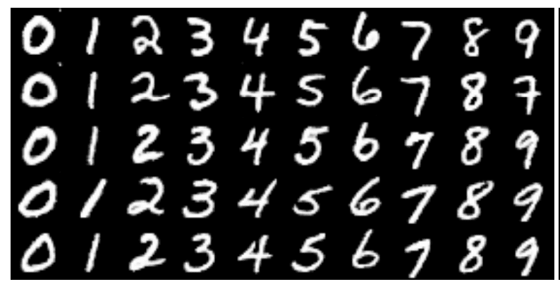
The paper explores two versions; the first uses just categorical control codes and allows the model to map one categorical variable to approximately one digit (although there is no ordering of the digits by categorical variables).
Example of Varying Generated Digit By Value of Categorical Control Code. Taken from the InfoGan paper.
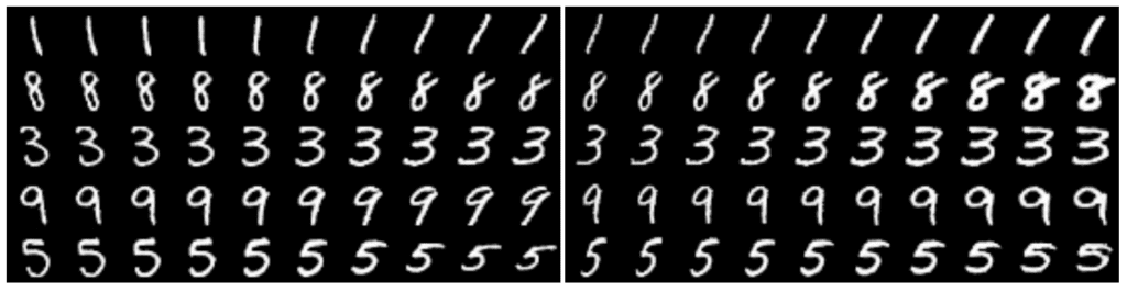
The paper also explores a version of the InfoGAN architecture with the one hot encoded categorical variable (c1) and two continuous control variables (c2 and c3).
The first continuous variable is discovered to control the rotation of the digits and the second controls the thickness of the digits.
Example of Varying Generated Digit Slant and Thickness Using Continuous Control Code. Taken from the InfoGan paper.
We will focus on the simpler case of using a categorical control variable with 10 values and encourage the model to learn to let this variable control the generated digit. You may want to extend this example by either changing the cardinality of the categorical control variable or adding continuous control variables.
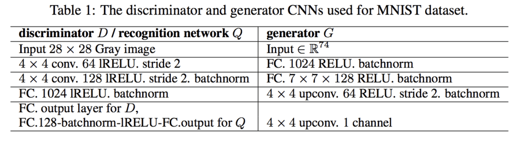
The configuration of the GAN model used for training on the MNIST dataset was provided as an appendix to the paper, reproduced below. We will use the listed configuration as a starting point in developing our own generator (g), discriminator (d), and auxiliary (q) models.
Summary of Generator, Discriminator and Auxiliary Model Configurations for the InfoGAN for Training MNIST. Taken from the InfoGan paper.
Let’s start off by developing the generator model as a deep convolutional neural network (e.g. a DCGAN).
The model could take the noise vector (z) and control vector (c) as separate inputs and concatenate them before using them as the basis for generating the image. Alternately, the vectors can be concatenated beforehand and provided to a single input layer in the model. The approaches are equivalent and we will use the latter in this case to keep the model simple.
The define_generator() function below defines the generator model and takes the size of the input vector as an argument.
A fully connected layer takes the input vector and produces a sufficient number of activations to create 512 7×7 feature maps from which the activations are reshaped. These then pass through a normal convolutional layer with 1×1 stride, then two subsequent upsamplings transpose convolutional layers with a 2×2 stride first to 14×14 feature maps then to the desired 1 channel 28×28 feature map output with pixel values in the range [-1,-1] via a tanh activation function.
Good generator configuration heuristics are as follows, including a random Gaussian weight initialization, ReLU activations in the hidden layers, and use of batch normalization.
Next, we can define the discriminator and auxiliary models.
The discriminator model is trained in a standalone manner on real and fake images, as per a normal GAN. Neither the generator nor the auxiliary models are fit directly; instead, they are fit as part of a composite model.
Both the discriminator and auxiliary models share the same input and feature extraction layers but differ in their output layers. Therefore, it makes sense to define them both at the same time.
Again, there are many ways that this architecture could be implemented, but defining the discriminator and auxiliary models as separate models first allows us later to combine them into a larger GAN model directly via the functional API.
The define_discriminator() function below defines the discriminator and auxiliary models and takes the cardinality of the categorical variable (e.g.number of values, such as 10) as an input. The shape of the input image is also parameterized as a function argument and set to the default value of the size of the MNIST images.
The feature extraction layers involve two downsampling layers, used instead of pooling layers as a best practice. Also following best practice for DCGAN models, we use the LeakyReLU activation and batch normalization.
The discriminator model (d) has a single output node and predicts the probability of an input image being real via the sigmoid activation function. The model is compiled as it will be used in a standalone way, optimizing the binary cross entropy function via the Adam version of stochastic gradient descent with best practice learning rate and momentum.
The auxiliary model (q) has one node output for each value in the categorical variable and uses a softmax activation function. A fully connected layer is added between the feature extraction layers and the output layer, as was used in the InfoGAN paper. The model is not compiled as it is not for or used in a standalone manner.
This model uses all submodels and is the basis for training the weights of the generator model.
The define_gan() function below implements this and defines and returns the model, taking the three submodels as input.
The discriminator is trained in a standalone manner as mentioned, therefore all weights of the discriminator are set as not trainable (in this context only). The output of the generator model is connected to the input of the discriminator model, and to the input of the auxiliary model.
This creates a new composite model that takes a [noise + control] vector as input, that then passes through the generator to produce an image. The image then passes through the discriminator model to produce a classification and through the auxiliary model to produce a prediction of the control variables.
The model has two output layers that need to be trained with different loss functions. Binary cross entropy loss is used for the discriminator output, as we did when compiling the discriminator for standalone use, and mutual information loss is used for the auxiliary model, which, in this case, can be implemented directly as categorical cross-entropy and achieve the desired result.
1
2
3
4
5
6
7
8
9
10
11
12
13
14
15
16
# define the combined discriminator, generator and q network model
def define_gan(g_model,d_model,q_model):
# make weights in the discriminator (some shared with the q model) as not trainable
Running the example creates all three models, then creates the composite GAN model and saves a plot of the model architecture.
Note: creating this plot assumes that the pydot and graphviz libraries are installed. If this is a problem, you can comment out the import statement and the call to the plot_model() function.
The plot shows all of the detail for the generator model and the compressed description of the discriminator and auxiliary models. Importantly, note the shape of the output of the discriminator as a single node for predicting whether the image is real or fake, and the 10 nodes for the auxiliary model to predict the categorical control code.
Recall that this composite model will only be used to update the model weights of the generator and auxiliary models, and all weights in the discriminator model will remain untrainable, i.e. only updated when the standalone discriminator model is updated.
Plot of the Composite InfoGAN Model for training the Generator and Auxiliary Models
Next, we will develop inputs for the generator.
Each input will be a vector comprised of noise and the control codes. Specifically, a vector of Gaussian random numbers and a one hot encoded randomly selected categorical value.
The generate_latent_points() function below implements this, taking as input the size of the latent space, the number of categorical values, and the number of samples to generate as arguments. The function returns the input concatenated vectors as input for the generator model, as well as the standalone control codes. The standalone control codes will be required when updating the generator and auxiliary models via the composite GAN model, specifically for calculating the mutual information loss for the auxiliary model.
1
2
3
4
5
6
7
8
9
10
11
12
13
# generate points in latent space as input for the generator
The MNIST dataset can be loaded, transformed into 3D input by adding an additional dimension for the grayscale images, and scaling all pixel values to the range [-1,1] to match the output from the generator model. This is implemented in the load_real_samples() function below.
We can retrieve batches of real samples required when training the discriminator by choosing a random subset of the dataset. This is implemented in the generate_real_samples() function below that returns the images and the class label of 1, to indicate to the discriminator that they are real images.
The discriminator also requires batches of fake samples generated via the generator, using the vectors from generate_latent_points() function as input. The generate_fake_samples() function below implements this, returning the generated images along with the class label of 0, to indicate to the discriminator that they are fake images.
1
2
3
4
5
6
7
8
9
10
11
12
13
14
15
16
17
18
19
20
21
22
23
24
25
26
27
28
29
30
31
32
# load images
def load_real_samples():
# load dataset
(trainX,_),(_,_)=load_data()
# expand to 3d, e.g. add channels
X=expand_dims(trainX,axis=-1)
# convert from ints to floats
X=X.astype('float32')
# scale from [0,255] to [-1,1]
X=(X-127.5)/127.5
print(X.shape)
returnX
# select real samples
def generate_real_samples(dataset,n_samples):
# choose random instances
ix=randint(0,dataset.shape[0],n_samples)
# select images and labels
X=dataset[ix]
# generate class labels
y=ones((n_samples,1))
returnX,y
# use the generator to generate n fake examples, with class labels
Next, we need to keep track of the quality of the generated images.
We will periodically use the generator to generate a sample of images and save the generator and composite models to file. We can then review the generated images at the end of training in order to choose a final generator model and load the model to start using it to generate images.
The summarize_performance() function below implements this, first generating 100 images, scaling their pixel values back to the range [0,1], and saving them as a plot of images in a 10×10 square.
The generator and composite GAN models are also saved to file, with a unique filename based on the training iteration number.
1
2
3
4
5
6
7
8
9
10
11
12
13
14
15
16
17
18
19
20
21
22
23
24
25
# generate samples and save as a plot and save the model
print('>Saved: %s, %s, and %s'%(filename1,filename2,filename3))
Finally, we can train the InfoGAN.
This is implemented in the train() function below that takes the defined models and configuration as arguments and runs the training process.
The models are trained for 100 epochs and 64 samples are used in each batch. There are 60,000 images in the MNIST training dataset, therefore one epoch involves 60,000/64, or 937 batches or training iterations. Multiplying this by the number of epochs, or 100, means that there will be a total of 93,700 total training iterations.
Each training iteration involves first updating the discriminator with half a batch of real samples and half a batch of fake samples to form one batch worth of weight updates, or 64, each iteration. Next, the composite GAN model is updated based on a batch worth of noise and control code inputs. The loss of the discriminator on real and fake images and the loss of the generator and auxiliary model is reported each training iteration.
We can then configure and create the models, then run the training process.
We will use 10 values for the single categorical variable to match the 10 known classes in the MNIST dataset. We will use a latent space with 64 dimensions to match the InfoGAN paper, meaning, in this case, each input vector to the generator model will be 64 (random Gaussian variables) + 10 (one hot encoded control variable) or 72 elements in length.
1
2
3
4
5
6
7
8
9
10
11
12
13
14
15
# number of values for the categorical control code
Tying this together, the complete example of training an InfoGAN model on the MNIST dataset with a single categorical control variable is listed below.
Running the example may take some time, and GPU hardware is recommended, but not required.
Note: Your results may vary given the stochastic nature of the algorithm or evaluation procedure, or differences in numerical precision. Consider running the example a few times and compare the average outcome.
The loss across the models is reported each training iteration. If the loss for the discriminator remains at 0.0 or goes to 0.0 for an extended time, this may be a sign of a training failure and you may want to restart the training process. The discriminator loss may start at 0.0, but will likely rise, as it did in this specific case.
The loss for the auxiliary model will likely go to zero, as it perfectly predicts the categorical variable. Loss for the generator and discriminator models is likely to hover around 1.0 eventually, to demonstrate a stable training process or equilibrium between the training of the two models.
1
2
3
4
5
6
7
8
9
10
11
12
>1, d[0.924,0.758], g[0.448] q[2.909]
>2, d[0.000,2.699], g[0.547] q[2.704]
>3, d[0.000,1.557], g[1.175] q[2.820]
>4, d[0.000,0.941], g[1.466] q[2.813]
>5, d[0.000,1.013], g[1.908] q[2.715]
...
>93696, d[0.814,1.212], g[1.283] q[0.000]
>93697, d[1.063,0.920], g[1.132] q[0.000]
>93698, d[0.999,1.188], g[1.128] q[0.000]
>93699, d[0.935,0.985], g[1.229] q[0.000]
>93700, d[0.968,1.016], g[1.200] q[0.001]
>Saved: generated_plot_93700.png, model_93700.h5, and gan_model_93700.h5
Plots and models are saved every 10 epochs or every 9,370 training iterations.
Reviewing the plots should show poor quality images in early epochs and improved and stable quality images in later epochs.
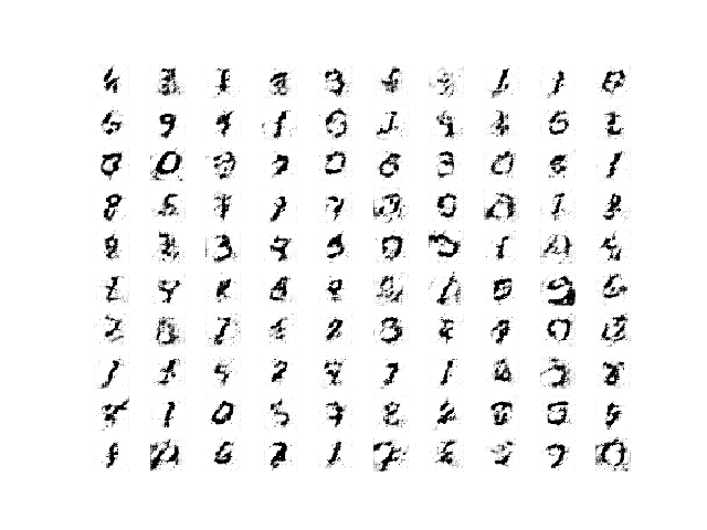
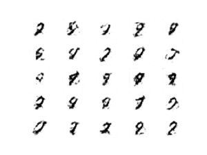
For example, the plot of images saved after the first 10 epochs is below showing low-quality generated images.
Plot of 100 Random Images Generated by the InfoGAN after 10 Training Epochs
More epochs does not mean better quality, meaning that the best quality images may not be those from the final model saved at the end of training.
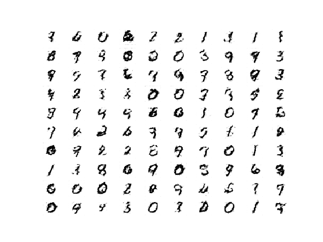
Review the plots and choose a final model with the best image quality. In this case, we will use the model saved after 100 epochs or 93,700 training iterations.
Plot of 100 Random Images Generated by the InfoGAN after 100 Training Epochs
How to Use Control Codes With a Trained InfoGAN Model
Now that we have trained the InfoGAN model, we can explore how to use it.
First, we can load the model and use it to generate random images, as we did during training.
The complete example is listed below.
Change the model filename to match the model filename that generated the best images during your training run.
1
2
3
4
5
6
7
8
9
10
11
12
13
14
15
16
17
18
19
20
21
22
23
24
25
26
27
28
29
30
31
32
33
34
35
36
37
38
39
40
41
42
43
44
45
46
47
48
49
50
51
# example of loading the generator model and generating images
from math import sqrt
from numpy import hstack
from numpy.random import randn
from numpy.random import randint
from keras.models import load_model
from keras.utils import to_categorical
from matplotlib import pyplot
# generate points in latent space as input for the generator
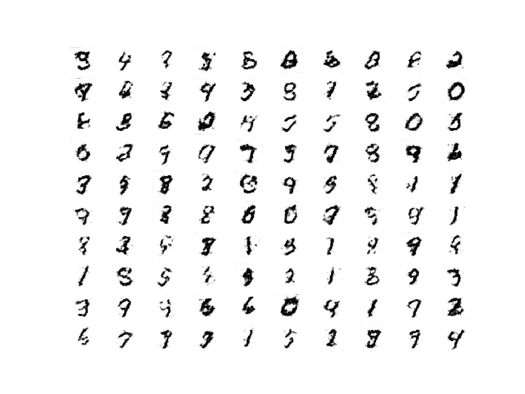
Running the example will load the saved generator model and use it to generate 100 random images and plot the images on a 10×10 grid.
Plot of 100 Random Images Created by Loading the Saved InfoGAN Generator Model
Next, we can update the example to test how much control our control variable gives us.
We can update the generate_latent_points() function to take an argument of the value for the categorical value in [0,9], encode it, and use it as input along with noise vectors.
1
2
3
4
5
6
7
8
9
10
11
12
13
# generate points in latent space as input for the generator
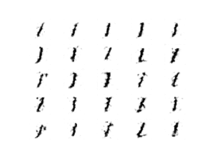
The result is a grid of 25 generated images generated with the categorical code set to the value 1.
Note: Your results may vary given the stochastic nature of the algorithm or evaluation procedure, or differences in numerical precision. Consider running the example a few times and compare the average outcome.
The values of the control code are expected to influence the generated images; specifically, they are expected to influence the digit type. They are not expected to be ordered though, e.g. control codes of 1, 2, and 3 to create those digits.
Nevertheless, in this case, the control code with a value of 1 has resulted in images generated that look like a 1.
Plot of 25 Images Generated by the InfoGAN Model With the Categorical Control Code Set to 1
Experiment with different digits and review what the value is controlling exactly about the image.
For example, setting the value to 5 in this case (digit = 5) results in generated images that look like the number “8“.
Plot of 25 Images Generated by the InfoGAN Model With the Categorical Control Code Set to 5
Extensions
This section lists some ideas for extending the tutorial that you may wish to explore.
Change Cardinality. Update the example to use different cardinality of the categorical control variable (e.g. more or fewer values) and review the effect on the training process and the control over generated images.
Uniform Control Variables. Update the example and add two uniform continuous control variables to the auxiliary model and review the effect on the training process and the control over generated images.
Gaussian Control Variables. Update the example and add two Gaussian continuous control variables to the auxiliary model and review the effect on the training process and the control over generated images.
If you explore any of these extensions, I’d love to know.
Post your findings in the comments below.
Further Reading
This section provides more resources on the topic if you are looking to go deeper.
In this tutorial, you discovered how to implement an Information Maximizing Generative Adversarial Network model from scratch.
Specifically, you learned:
The InfoGAN is motivated by the desire to disentangle and control the properties in generated images.
The InfoGAN involves the addition of control variables to generate an auxiliary model that predicts the control variables, trained via mutual information loss function.
How to develop and train an InfoGAN model from scratch and use the control variables to control which digit is generated by the model.
Do you have any questions?
Ask your questions in the comments below and I will do my best to answer.
Hey Darrren,
Could you manage to make it work?
I am trying and I have a similar model as Jason has posted below..but am not able to get it working.
I’m actually trying to implement a continuous variable to an ACGAN.
Is it possible to build InfoGAN along with a classifier? I understand that InfoGAN can generate a desired class of image with the control variable, but at the same time, I want to input an unseen MNIST data and see if the model correctly classifies them.
Yes, I constructed an InfoGAN model using your code. But what I want to do now is to input an unseen MNIST image into the generator in the reverse direction and see where it locates in the learned latent space. Basically, I wish to visualize the latent space that the model learnt so that when new data is input, it is first classified its class and then shown on the latent space. Would that be possible?
David, a neural network is a consecutive application of operations, such as affine transforms Wx + b and activation functions. If all of these are invertible (weight matrix W usually is), then the whole operation is invertible.
In this particular code, the ‘relu’ activation function is used, it is not invertible since it multiplies something by 0 half of the time. LeakyReLU is invertible, as well as some other activation functions.
You can however go a different path and try constructing an autoencoder network, where the decoder part is the generator function that you’ve trained already. You would train it by freezing the decoder and feeding the same image on inputs and outputs, the training data could come from the pre-trained generator network.
The result should be a combination of encoder+decoder where, when fed an image, the encoder would produce latent variables which would produce the same image when fed into the GAN generator (decoder).
Thank you very much for your reply. However, my concerns are similar to those of David’s above, i.e., how to achieve the unsupervised classification of data on the InfoGAN trained classifier. So far I have not found any implementation of InfoGAN that meets the requirements.
Anyway, I’ve learned a lot from your amazing tutorial, thank you very much.
But actually my generated images are not good no matter it runs 100 epochs or 1000 epochs.
I think it is the training process of q_net make it sick.
May be we can try to pull the independent part of the q_net out of the Discriminator, then set the shared part q_model.trainable=False. That achieves great images.
I am little bit confused. Do you mean:
– define d_net and q_net in the same way as done in this great tutorial.
– make d_net part of q_net non-trainable.
– train q_net with real data (real images with its corresponding labels).
Hi Jason, Thanks for the info gan code.
the loss function of info gen is as follows,
min max V(D, G)= V (D, G) − λI(c; G(z, c))
G D
you considered λ=1 , but how does ‘categorical cross-entropy loss’ on q_model equals mutual information between c and G(z,c) ?????
Hi! great tutorial.
May i ask, why did you train the Q model with the G model.
why not using a CNN in Q model and train it separately like the D model?
I understand but do you think that applying these changes is reasonable, and it might work?
I am already trying to apply this model, but I am trying to check if my logic and way of thinking are in place.
Here is the list of changes I am making:
– change the Q model to a CNN model.
– train the Q model separately.
Thanks for your help.
Hi again!
So I trained the model you published on google colab, and I am seeing this:
> 49943, d[0.000,0.000], g[0.000] q[0.000]
This is epoch 40 or 50, and the loss is 0!?
In addition to that, the generated images are awful. Any idea why?
So, I tried several changes, and somehow removing the batch normalization solved my problem.
I tried adding batch normalisation to vanilla DCGAN(for MNIST) and the same thing happened.
It seems like batch normalization is not a good addition to GANs, and yet I always read recommendations about adding it. I am confused.
Did you experience the same thing?
Hello again Dr.
So I after some experimentation the continuous control variables model worked.
I used two control variables model just as you, I also removed the batch normalization.
But I noticed that the model that has extra variables (categorical or continuous) had a higher chance of generating wrong the wrong digit. Also, the two continuous variables had the effect of thickness and width. Somehow digits with lower width turn into “1” so maybe he is not generating the wrong digit, after all, hard to tell…
Sorry for butchering the language, I am still hyped.
Also, I tried the same concept on the CelebFaces dataset, I chose one categorical variable with two categories(kind of man and women), I thought that the model will learn the characteristics and the random noise will shape the details of the faces. Unfortunately, that did not work out, i got two types of faces every time, in green colour but not what I was looking for, here is the models and results: https://drive.google.com/drive/folders/1GMom1tIltHbph-Rr4Qdt1Vg9wal4rWJ3?usp=sharing
So my question is how would you make an infoGAN for human faces and what variables would you use.
Thank you.
Yes, a conditional GAN such as an infogan would be a good approach for generating men/women faces. A categorical variable could be used and the generator would have to be good enough/big enough to generate realistic faces.
Perhaps borrow the architecture for the generator from another model that is already good at generating faces.
Hi Jason,
Please correct me if I am wrong.
i) In the implementation, did you generate two fake batches, one for updating Discriminator, one for updating the auxiliary network?
ii) In the original InfoGAN implementation, it seems that the discriminator was not frozen during the update for the auxiliary network?
Thanks!
Then it seems that you updated your composite gan model (generator, and the q model) with another batch of newly generated fake data (correct me if I’m wrong):
z_input, cat_codes, con_codes = generate_latent_points(latent_dim, n_cat, n_con, n_batch)
# create inverted labels for the fake samples
y_gan = ones((n_batch, 1))
# update the g via the d and q error
_,g_1,g_2,g3 = gan_model.train_on_batch(z_input, [y_gan, cat_codes, con_codes])
ii) I am not familiar with Keras, so I don’t know when you make the Discriminator parameters untrainable, whether the shared layers with the Q model are also made untrainable (in other words, whether the Discriminator and Q model keep separate copies of the shared layers). I think the original infoGAN intended that the shared layers are updatable for by both D and Q (only one copy accessed and updated by both D and Q). When you are updating the Generator (fixing Discriminator for sure) and updating the Q model, two case will happen:
i. if I guessed it right that the shared layers are not updated when you update the Q model, then this is not what the original paper intended.
ii. if I guessed it wrong that the shared layers are actually updated when you update the Q model, then your implementation is correct.
Please inform, thanks!
Best
The combined model is how we update the gan model _via_ the discriminator model. The discriminator remains unchanged in this case – the shared layers are not updated.
To clarify my point a bit: the shared layers should be updated in the Q model’s perspective (when you update the composite gan model), even though the discriminator is fixed.
I was eventually able to get it working with TensorFlow 2.5.0. Now I am attempting to add more control variables – such as ones for width/angle. Any resources/tips on how to do this?


 From Scratch with Keras")


Nice. This is the same as AC-GAN right ? (Auxiliar classifier gan)
I have this implementation : https://raw.githubusercontent.com/rjpg/bftensor/master/Autoencoder/src/ac-gan2.py
To Control what classe to generate I multiply noise (latent) by the number of the class. Also called “give color to noise”. And it works.
But your implementation is very elegant Nice work.
No, InfoGAN is different from AC-GAN covered here:
https://machinelearningmastery.com/how-to-develop-an-auxiliary-classifier-gan-ac-gan-from-scratch-with-keras/
Hi Jason,
Is it possible for me to get some code snippets of how to do the continuous control variables?
Thanks,
Darren
Yeah, I tried for about 10 minutes and it sucked. I recommend using the approach in the paper instead of my terrible approach.
Nevertheless, here it is for completeness:
If you figure out how to get good results with it, please let me know.
Hey Darrren,
Could you manage to make it work?
I am trying and I have a similar model as Jason has posted below..but am not able to get it working.
I’m actually trying to implement a continuous variable to an ACGAN.
Thanks in advance,
Caterina
Hi Jason, thanks a lot for your work.
Is it possible to build InfoGAN along with a classifier? I understand that InfoGAN can generate a desired class of image with the control variable, but at the same time, I want to input an unseen MNIST data and see if the model correctly classifies them.
Thanks
Generally GANs are designed for image synthesis, not classification.
If you need a classification model, see this post:
https://machinelearningmastery.com/how-to-develop-a-convolutional-neural-network-from-scratch-for-mnist-handwritten-digit-classification/
Yes, I constructed an InfoGAN model using your code. But what I want to do now is to input an unseen MNIST image into the generator in the reverse direction and see where it locates in the learned latent space. Basically, I wish to visualize the latent space that the model learnt so that when new data is input, it is first classified its class and then shown on the latent space. Would that be possible?
That sounds fun.
Sorry, I don’t have an example of this, some experiments/prototyping will be required to figure out how. Let me know how you go.
Could you save the weights of the model, construct a “reverse” model and load the weights onto that layer by layer?
David, a neural network is a consecutive application of operations, such as affine transforms Wx + b and activation functions. If all of these are invertible (weight matrix W usually is), then the whole operation is invertible.
In this particular code, the ‘relu’ activation function is used, it is not invertible since it multiplies something by 0 half of the time. LeakyReLU is invertible, as well as some other activation functions.
You can however go a different path and try constructing an autoencoder network, where the decoder part is the generator function that you’ve trained already. You would train it by freezing the decoder and feeding the same image on inputs and outputs, the training data could come from the pre-trained generator network.
The result should be a combination of encoder+decoder where, when fed an image, the encoder would produce latent variables which would produce the same image when fed into the GAN generator (decoder).
Hi David, I’m also studying about the problem you proposed, have you found any approaches to have the unseen MNIST data classified?
Try this:
https://machinelearningmastery.com/how-to-develop-a-convolutional-neural-network-from-scratch-for-mnist-handwritten-digit-classification/
Thank you very much for your reply. However, my concerns are similar to those of David’s above, i.e., how to achieve the unsupervised classification of data on the InfoGAN trained classifier. So far I have not found any implementation of InfoGAN that meets the requirements.
Anyway, I’ve learned a lot from your amazing tutorial, thank you very much.
It sounds like you’re interested in “clustering” that is unsupervised rather than “classification” that is supervised.
The above example is something in between, called “semi-supervised” that does a little clustering and a little classification.
Hi Jason, thanks your article.
But actually my generated images are not good no matter it runs 100 epochs or 1000 epochs.
I think it is the training process of q_net make it sick.
May be we can try to pull the independent part of the q_net out of the Discriminator, then set the shared part q_model.trainable=False. That achieves great images.
Fair enough.
Hi lei!
I am little bit confused. Do you mean:
– define d_net and q_net in the same way as done in this great tutorial.
– make d_net part of q_net non-trainable.
– train q_net with real data (real images with its corresponding labels).
Did I understand your approach correctly?
Thank you in advance
Hi Jason, Thanks for the info gan code.
the loss function of info gen is as follows,
min max V(D, G)= V (D, G) − λI(c; G(z, c))
G D
you considered λ=1 , but how does ‘categorical cross-entropy loss’ on q_model equals mutual information between c and G(z,c) ?????
I believe we go through this in section “How to Implement the InfoGAN Loss Function”.
yeah, it was clearly explained. Thank you so much.
You’re welcome.
Hi! great tutorial.
May i ask, why did you train the Q model with the G model.
why not using a CNN in Q model and train it separately like the D model?
I designed the implementation to match the intent of the paper.
I understand but do you think that applying these changes is reasonable, and it might work?
I am already trying to apply this model, but I am trying to check if my logic and way of thinking are in place.
Here is the list of changes I am making:
– change the Q model to a CNN model.
– train the Q model separately.
Thanks for your help.
Hard to know, perhaps try it and see.
For sure, thank you so much!
You’re welcome.
Hi again!
So I trained the model you published on google colab, and I am seeing this:
> 49943, d[0.000,0.000], g[0.000] q[0.000]
This is epoch 40 or 50, and the loss is 0!?
In addition to that, the generated images are awful. Any idea why?
Sorry, what I meant is, I run the code you shared on this post on google colab.
A loss of zero suggest a mode failure:
https://machinelearningmastery.com/practical-guide-to-gan-failure-modes/
Perhaps try training the model again.
So, I tried several changes, and somehow removing the batch normalization solved my problem.
I tried adding batch normalisation to vanilla DCGAN(for MNIST) and the same thing happened.
It seems like batch normalization is not a good addition to GANs, and yet I always read recommendations about adding it. I am confused.
Did you experience the same thing?
Well done!
It really depends on the specific data and model being used. Often batch norm is not needed for simple dcgans.
I agree. Thank you so much Sir!
You’re welcome.
Hello again Dr.
So I after some experimentation the continuous control variables model worked.
I used two control variables model just as you, I also removed the batch normalization.
But I noticed that the model that has extra variables (categorical or continuous) had a higher chance of generating wrong the wrong digit. Also, the two continuous variables had the effect of thickness and width. Somehow digits with lower width turn into “1” so maybe he is not generating the wrong digit, after all, hard to tell…
Sorry for butchering the language, I am still hyped.
Here is a link to the saved models: https://drive.google.com/drive/folders/1Gv3fyAi8oypC3JhTdCmc6CxOIdqHJKeA?usp=sharing
Here is a link to my collab playground:
https://colab.research.google.com/drive/13B4COwR-UktpQ7pTQntORri2jwn13BuQ?usp=sharing
Also, I tried the same concept on the CelebFaces dataset, I chose one categorical variable with two categories(kind of man and women), I thought that the model will learn the characteristics and the random noise will shape the details of the faces. Unfortunately, that did not work out, i got two types of faces every time, in green colour but not what I was looking for, here is the models and results:
https://drive.google.com/drive/folders/1GMom1tIltHbph-Rr4Qdt1Vg9wal4rWJ3?usp=sharing
So my question is how would you make an infoGAN for human faces and what variables would you use.
Thank you.
Well done on your experiments!
Yes, a conditional GAN such as an infogan would be a good approach for generating men/women faces. A categorical variable could be used and the generator would have to be good enough/big enough to generate realistic faces.
Perhaps borrow the architecture for the generator from another model that is already good at generating faces.
Hi Jason,
Please correct me if I am wrong.
i) In the implementation, did you generate two fake batches, one for updating Discriminator, one for updating the auxiliary network?
ii) In the original InfoGAN implementation, it seems that the discriminator was not frozen during the update for the auxiliary network?
Thanks!
The discriminator is updated on real and fake images.
The discriminator weights are not frozen, they are only not updated when updating the generator – e.g. typical for gan updates.
Perhaps this will help if you are new to the gan training implementation:
https://machinelearningmastery.com/how-to-code-the-generative-adversarial-network-training-algorithm-and-loss-functions/
Thank you.
I know the how the generator and discriminator are updated in a GAN.
i) In your code, you first updated the discriminator and q model through real and fake images:
# get randomly selected ‘real’ samples
X_real, y_real = generate_real_samples(dataset, half_batch)
# update discriminator and q model weights
d_loss1 = d_model.train_on_batch(X_real, y_real)
# generate ‘fake’ examples
X_fake, y_fake = generate_fake_samples(g_model, latent_dim, n_cat, n_con, half_batch)
# update discriminator model weights
d_loss2 = d_model.train_on_batch(X_fake, y_fake)
Then it seems that you updated your composite gan model (generator, and the q model) with another batch of newly generated fake data (correct me if I’m wrong):
z_input, cat_codes, con_codes = generate_latent_points(latent_dim, n_cat, n_con, n_batch)
# create inverted labels for the fake samples
y_gan = ones((n_batch, 1))
# update the g via the d and q error
_,g_1,g_2,g3 = gan_model.train_on_batch(z_input, [y_gan, cat_codes, con_codes])
ii) I am not familiar with Keras, so I don’t know when you make the Discriminator parameters untrainable, whether the shared layers with the Q model are also made untrainable (in other words, whether the Discriminator and Q model keep separate copies of the shared layers). I think the original infoGAN intended that the shared layers are updatable for by both D and Q (only one copy accessed and updated by both D and Q). When you are updating the Generator (fixing Discriminator for sure) and updating the Q model, two case will happen:
i. if I guessed it right that the shared layers are not updated when you update the Q model, then this is not what the original paper intended.
ii. if I guessed it wrong that the shared layers are actually updated when you update the Q model, then your implementation is correct.
Please inform, thanks!
Best
The combined model is how we update the gan model _via_ the discriminator model. The discriminator remains unchanged in this case – the shared layers are not updated.
You can learn more about this here:
https://machinelearningmastery.com/how-to-code-the-generative-adversarial-network-training-algorithm-and-loss-functions/
And here:
https://keras.io/getting_started/faq/#how-can-i-freeze-layers-and-do-finetuning
Thank you Jason.
If the shared layers are not updated, then I am afraid this is not what the original implementation intended: https://github.com/openai/InfoGAN/blob/master/infogan/algos/infogan_trainer.py
I believe the implementation is correct, perhaps we’re talking past each other.
To clarify my point a bit: the shared layers should be updated in the Q model’s perspective (when you update the composite gan model), even though the discriminator is fixed.
What version of TensorFlow was used to run the code provided in this tutorial? I can’t seem to get it working with 2.8 or 2.6
Hi Daniel…What error messages or issues are you experiencing?
I was eventually able to get it working with TensorFlow 2.5.0. Now I am attempting to add more control variables – such as ones for width/angle. Any resources/tips on how to do this?
Hi Daniel…The following may be of interest to you:
https://theailearner.com/tag/control-variables-gan/