Data Cleaning and Preparation for Machine Learning
Data cleaning and preparation is a critical first step in any machine learning project. Although we often think of data scientists as spending lots of time tinkering with algorithms and machine learning models, the reality is that most data scientists spend most of their time cleaning data.
In this blog post (originally written by Dataquest student Daniel Osei and updated by Dataquest in June 2019) we'll walk through the process of data cleaning in Python, examining a data set, selecting columns for features, exploring the data visually and then encoding the features for machine learning.
We suggest using a Jupyter Notebook to follow along with this tutorial.
To learn more about data cleaning, check out one of our interactive data cleaning courses:
- Data Cleaning and Analysis course (Python)
- Advanced Data Cleaning course (Python)
- Data Cleaning (R)
Understanding the Data
Before we start cleaning data for a machine learning project, it is vital to understand what the data is, and what we want to achieve. Without that understanding, we have no basis from which to make decisions about what data is relevant as we clean and prepare our data.
We'll be working with some data from Lending Club, a marketplace for personal loans that matches borrowers who are seeking a loan with investors looking to lend money and make a return. Each borrower fills out a comprehensive application, providing their past financial history, the reason for the loan, and more. Lending Club evaluates each borrower's credit score using past historical data (and their own data science process!) and assigns an interest rate to the borrower.
Approved loans are listed on the Lending Club website, where qualified investors can browse recently approved loans, the borrower's credit score, the purpose for the loan, and other information from the application.
Once an investor decides to fund a loan, the borrower then makes monthly payments back to Lending Club. Lending Club redistributes these payments to investors. This means that investors don't have to wait until the full amount is paid off to start to see returns. If a loan is fully paid off on time, the investors make a return which corresponds to the interest rate the borrower had to pay in addition to the requested amount.
Many loans aren't completely paid off on time, however, and some borrowers default on the loan. That's the problem we'll be trying to address as we clean some data from Lending Club for machine learning. Let's imagine we've been tasked with building a model to predict whether borrowers are likely to pay or default on their loans.
Step 1: Examining the Data Set
Lending Club periodically releases data for all its approved and declined loan applicationson their website. To ensure we're all working with the same set of data, we've mirrored the data we'll be using for this tutorial on data.world.
On LendingClub's site, you can select different year ranges to download data sets (in CSV format) for both approved and declined loans. You'll also find a data dictionary (in XLS format) towards the bottom of the LendingClub page, which contains information on the different column names. This data dictionary is useful for understanding what each column represents in the data set. The data dictionary contains two sheets:
- LoanStats sheet: describes the approved loans dataset
- RejectStats sheet: describes the rejected loans dataset
We'll be using the LoanStats sheet since we're interested in the approved loans data set.
The approved loans data set contains information on current loans, completed loans, and defaulted loans. In this tutorial, we'll be working with approved loans data for the years 2007 to 2011, but similar cleaning steps would be required for any of the data posted to LendingClub's site.
First, lets import some of the libraries that we'll be using, and set some parameters to make the output easier to read. For the purposes of this tutorial, we'll be assuming a solid grasp of the fundamentals of working with data in Python, including using pandas, numpy, etc., so if you need to brush up on any of those skills you may want to browse our course listings.
import pandas as pd
import numpy as np
pd.set_option('max_columns', 120)
pd.set_option('max_colwidth', 5000)
import matplotlib.pyplot as plt
import seaborn as sns
Loading The Data Into Pandas
We've downloaded our data set and named it lending_club_loans.csv, but now we need to load it into a pandas DataFrame to explore it. Once it's loaded, we'll want to do some basic cleaning tasks to remove some information we don't need that will make our data processing slower.
Specifically, we're going to:
- Remove the first line: it contains extraneous text instead of the column titles. This text prevents the data set from being parsed properly by the pandas library.
- Remove the 'desc' column: it contains a long text explanation for the loan that we won't need.
- Remove the 'url' column: it contains a link to each on Lending Club which can only be accessed with an investor account.
- Removing all columns with more than 50% missing values: This will allow us to work faster (and our data set is large enough that it will still be meaningful without them.
We'll also name the filtered data set loans_2007, and at the end of this section we'll save it as loans_2007.csv to keep it separate from the raw data. This is good practice and makes sure we have our original data in case we need to go back and retrieve any of the things we're removing.
Now, let's go ahead and perform these steps:
# skip row 1 so pandas can parse the data properly.
loans_2007 = pd.read_csv('data/lending_club_loans.csv', skiprows=1, low_memory=False)
half_count = len(loans_2007) / 2
loans_2007 = loans_2007.dropna(thresh=half_count,axis=1) # Drop any column with more than 50% missing values
loans_2007 = loans_2007.drop(['url','desc'],axis=1) # These columns are not useful for our purposes
Let's use the pandas head() method to display first three rows of the loans_2007 DataFrame, just to make sure we were able to load the dataset properly:
loans_2007.head(3)Let's also use pandas .shape attribute to view the number of samples and features we're dealing with at this stage:
loans_2007.shape(42538, 56)Step 2: Narrowing Down Our Columns for Cleaning
Now that we've got our data set up, we should spend some time exploring it and understanding what feature each column represents. This is important, because having a poor understanding of the features could cause us to make mistakes in the data analysis and the modeling process.
We'll be using the data dictionary LendingClub provides to help us become familiar with the columns and what each represents in the data set. To make the process easier, we'll create a DataFrame to contain the names of the columns, data type, first row's values, and description from the data dictionary. To make this easier, we've pre-converted the data dictionary from Excel format to a CSV.
Let's load that dictionary and take a look.
data_dictionary = pd.read_csv('LCDataDictionary.csv') # Loading in the data dictionary
print(data_dictionary.shape[0])
print(data_dictionary.columns.tolist())
117
['LoanStatNew', 'Description']
data_dictionary.head()
data_dictionary = data_dictionary.rename(columns={'LoanStatNew': 'name', 'Description': 'description'})Now that we've got the data dictionary loaded, let's join the first row of loans_2007 to the data_dictionary DataFrame to give us a preview DataFrame with the following columns:
name— contains the column names ofloans_2007.dtypes— contains the data types of theloans_2007columns.first value— contains the values ofloans_2007first row.description— explains what each column inloans_2007represents.
loans_2007_dtypes = pd.DataFrame(loans_2007.dtypes,columns=['dtypes'])
loans_2007_dtypes = loans_2007_dtypes.reset_index()
loans_2007_dtypes['name'] = loans_2007_dtypes['index']
loans_2007_dtypes = loans_2007_dtypes[['name','dtypes']]
loans_2007_dtypes['first value'] = loans_2007.loc[0].values
preview = loans_2007_dtypes.merge(data_dictionary, on='name',how='left')
preview.head()When we printed the shape of loans_2007 earlier, we noticed that it had 56 columns, so we know that this preview DataFrame has 56 rows (one explaining each column in loans_2007).
It can be cumbersome to try to explore all the rows of a preview at once, so instead we'll break it up into three parts and look at smaller selection of features each time. As we explore the features to better understand each of them, we'll want to pay attention to any column that:
- leaks information from the future (after the loan has already been funded),
- doesn't affect the borrower's ability to pay back the loan (e.g. a randomly generated ID value by Lending Club),
- is formatted poorly,
- requires more data or a lot of pre-processing to turn into useful a feature, or
- contains redundant information.
These are all things we'll want to be careful about, since handling them incorrectly will hurt our analysis in the long run.
We need to especially pay close attention to data leakage, which can cause the model to overfit. This is because the model would be also learning from features that won't be available when we're using it make predictions about future loans. We need to be sure our model is trained using only the data it would have at the point of a loan application.
First Group Of Columns
Let's display the first 19 rows of preview and analyze them:
preview[:19]After analyzing the columns and considering the model we're trying to build, we can conclude that the following features can be removed:
id— randomly generated field by LendingClub for unique identification purposes only.member_id— also randomly generated field by LendingClub for identification purposes only.funded_amnt— leaks information from the future (after the loan is already started to be funded).funded_amnt_inv— also leaks data from the future.sub_grade— contains redundant information that is already in thegradecolumn (more below).int_rate— also included within thegradecolumn.emp_title— requires other data and a lot of processing to become potentially usefulissued_d— leaks data from the future.
Note: Lending Club uses a borrower's grade and payment term (30 or months) to assign an interest rate (you can read more about Rates & Fees). This causes variations in interest rate within a given grade.
What may be useful for our model is to focus on clusters of borrowers instead of individuals. And, that's exactly what grading does — it segments borrowers based on their credit score and other behaviors, which is why we will keep the grade column and drop interest int_rate and sub_grade. Let's drop these columns from the DataFrame before moving onto to the next group of columns.
drop_list = ['id','member_id','funded_amnt','funded_amnt_inv',
'int_rate','sub_grade','emp_title','issue_d']
loans_2007 = loans_2007.drop(drop_list,axis=1)
Now we're ready to move on to the next group of columns (features).
Second Group Of Columns
Let's move on to the next 19 columns:
preview[19:38]In this group, take note of the fico_range_low and fico_range_high columns. While both are in the table above, we'll talk more about them after looking at the last group of columns. Also note that if you're working with newer LendingClub data, it may not include data on FICO scores.
For now, reviewing our second group of columns, we can further refine our data set by dropping the following columns:
zip_code- mostly redundant with the addr_state column since only the first 3 digits of the 5 digit zip code are visible.out_prncp- leaks data from the future.out_prncp_inv- also leaks data from the future.total_pymnt- also leaks data from the future.total_pymnt_inv- also leaks data from the future.
Let's go ahead and remove these 5 columns from the DataFrame:
drop_cols = [ 'zip_code','out_prncp','out_prncp_inv',
'total_pymnt','total_pymnt_inv']
loans_2007 = loans_2007.drop(drop_cols, axis=1)
Third Group Of Columns
Let's analyze the last group of features:
preview[38:]In this last group of columns, we need to drop the following, all of which leak data from the future:
total_rec_prncptotal_rec_inttotal_rec_late_feerecoveriescollection_recovery_feelast_pymnt_dlast_pymnt_amnt
Let's drop our last group of columns:
drop_cols = ['total_rec_prncp','total_rec_int',
'total_rec_late_fee','recoveries',
'collection_recovery_fee', 'last_pymnt_d'
'last_pymnt_amnt']
loans_2007 = loans_2007.drop(drop_cols, axis=1)
Great! We've now got a data set that's going to be much more useful for building our model, since it won't have to waste time processing irrelevant data and it won't be "cheating" by analyzing information from the future that gives away the loan's outcome.
Investigating FICO Score Columns
It's worth taking a moment to discuss the fico_range_low, fico_range_high, last_fico_range_low, and last_fico_range_high columns.
FICO scores are a credit score: a number used by banks and credit cards to represent how credit-worthy a person is. While there are a few types of credit scores used in the United States, the FICO score is the best known and most widely used.
When a borrower applies for a loan, LendingClub gets the borrower's credit score from FICO — they are given a lower and upper limit of the range that the borrowers score belongs to, and they store those values as fico_range_low, fico_range_high. After that, any updates to the borrowers score are recorded as last_fico_range_low, and last_fico_range_high.
A key part of any data science project is to do everything you can to understand the data. While researching this particular data set, I found a project from 2014 by a group of students from Stanford University. In However, following this group's project, another group from Stanford worked on this same Lending Club dataset. They used the FICO score columns, dropping only last_fico_range_low, in their modeling. This second group's report described last_fico_range_high as the one of the more important features in predicting accurate results.
With this information, the question we must answer is: do the FICO credit scores leak information from the future? Recall a column is considered to leak information when the data it contains won't be available when we use our model to make predictions — in this case when we use our model on future loan applications to predict whether a borrower will default.
This blog post (no longer available) examines in-depth the FICO scores for LendingClub loans, and notes that while looking at the trend of the FICO scores is a great predictor of whether a loan will default, FICO scores continue to be updated by LendingClub after a loan is funded. In other words, while we can use the initial FICO scores (fico_range_low and fico_range_high) — those would be available as part of a borrower's applicaton — we cannot use last_fico_range_low, and last_fico_range_high, as LendingClub may have updated these after the borrower's application.
Lets take a look at the values in the two columns we can use:
print(loans_2007['fico_range_low'].unique())
print(loans_2007['fico_range_high'].unique())
[ 735. 740. 690. 695. 730. 660. 675. 725. 710. 705. 720. 665. 670. 760. 685. 755. 680. 700. 790. 750. 715. 765. 745. 770. 780. 775. 795. 810. 800. 815. 785. 805. 825. 820. 630. 625. nan 650. 655. 645. 640. 635. 610. 620. 615.]
[ 739. 744. 694. 699. 734. 664. 679. 729. 714. 709. 724. 669. 674. 764. 689. 759. 684. 704. 794. 754. 719. 769. 749. 774. 784. 779. 799. 814. 804. 819. 789. 809. 829. 824. 634. 629. nan 654. 659. 649. 644. 639. 614. 624. 619.]
Let's get rid of the missing values, then plot histograms to look at the ranges of the two columns:
fico_columns = ['fico_range_high','fico_range_low']
print(loans_2007.shape[0])
loans_2007.dropna(subset=fico_columns,inplace=True)
print(loans_2007.shape[0])
loans_2007[fico_columns].plot.hist(alpha=0.5,bins=20);
42538
42535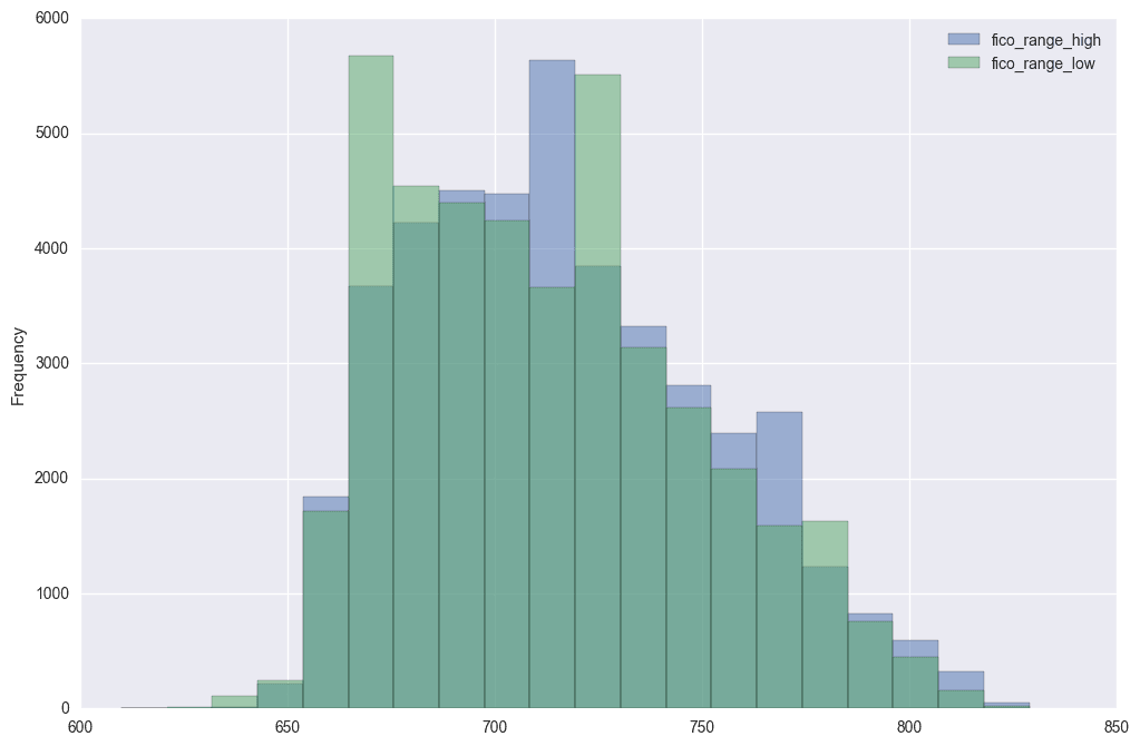
Let's now go ahead and create a column for the average of fico_range_low and fico_range_high columns and name it fico_average. Note that this is not the average FICO score for each borrower, but rather an average of the high and low range that we know the borrower is in.
loans_2007['fico_average'] = (loans_2007['fico_range_high'] + loans_2007['fico_range_low']) / 2Let's check what we just did.
cols = ['fico_range_low','fico_range_high','fico_average']
loans_2007[cols].head()Good! We got the mean calculations and everything right. Now, we can go ahead and drop fico_range_low, fico_range_high, last_fico_range_low, and last_fico_range_high columns.
drop_cols = ['fico_range_low','fico_range_high','last_fico_range_low', 'last_fico_range_high']
loans_2007 = loans_2007.drop(drop_cols, axis=1)
loans_2007.shape
(42535, 33)Notice just by becoming familiar with the columns in the data set, we've been able to reduce the number of columns from 56 to 33 without losing any meaningful data for our model. We've also avoided problems by dropping data that leaks information from the future, which would have messed up our model's results. This is why data cleaning is so important!
Decide On A Target Column
Now, we'll decide on the appropriate column to use as a target column for modeling.
Our main goal is predict who will pay off a loan and who will default, we we need to find a column that reflects this. We learned from the description of columns in the preview DataFrame that loan_status is the only field in the main data set that describes a loan status, so let's use this column as the target column.
preview[preview.name == 'loan_status']Currently, this column contains text values that need to be converted to numerical values to be able use for training a model. Let's explore the different values in this column and come up with a strategy for converting them. We'll use the DataFrame method value_counts() to return the frequency of the unique values in the loan_status column.
loans_2007["loan_status"].value_counts()
Fully Paid 33586
Charged Off 5653
Does not meet the credit policy. Status:Fully Paid 1988
Does not meet the credit policy. Status:Charged Off 761
Current 513
In Grace Period 16
Late (31-120 days) 12
Late (16-30 days) 5
Default 1
Name: loan_status, dtype: int64
The loan status has nine different possible values! Let's learn about these unique values to determine the ones that best describe the final outcome of a loan, and also the kind of classification problem we'll be dealing with.
We can read about most of the different loan statuses on the LendingClub website as well as these posts on the Lend Academy and Orchard forums.
Below, we'll pull that data together in a table below so we can see the unique values, their frequency in the data set, and get a clearer idea of what each means:
meaning = [
"Loan has been fully paid off.",
"Loan for which there is no longer a reasonable expectation of further payments.",
"While the loan was paid off, the loan application today would no longer meet the credit policy and wouldn't be approved on to the marketplace.",
"While the loan was charged off, the loan application today would no longer meet the credit policy and wouldn't be approved on to the marketplace.",
"Loan is up to date on current payments.",
"The loan is past due but still in the grace period of 15 days.",
"Loan hasn't been paid in 31 to 120 days (late on the current payment).",
"Loan hasn't been paid in 16 to 30 days (late on the current payment).",
"Loan is defaulted on and no payment has been made for more than 121 days."]
status, count = loans_2007["loan_status"].value_counts().index, loans_2007["loan_status"].value_counts().values
loan_statuses_explanation = pd.DataFrame({'Loan Status': status,'Count': count,'Meaning': meaning})[['Loan Status','Count','Meaning']]
loan_statuses_explanationRemember, our goal is to build a machine learning model that can learn from past loans in trying to predict which loans will be paid off and which won't. From the above table, only the Fully Paid and Charged Off values describe the final outcome of a loan. The other values describe loans that are still ongoing, and even though some loans are late on payments, we can't jump the gun and classify them as Charged Off.
Also, while the Default status resembles the Charged Off status, in LendingClub's eyes, loans that are charged off have essentially no chance of being repaid, while defaulted loans have a small chance. Therefore, we should use only samples where the loan_status column is 'Fully Paid' or 'Charged Off'.
We're not interested in any statuses that indicate that the loan is ongoing or in progress, because predicting that something is in progress doesn't tell us anything.
We're interested in being able to predict which of 'Fully Paid' or 'Charged Off' a loan will fall under, so we can treat the problem as binary classification. Let's remove all the loans that don't contain either 'Fully Paid' or 'Charged Off' as the loan's status and then transform the 'Fully Paid' values to 1 for the positive case and the 'Charged Off' values to 0 for the negative case.
This will mean that out of the ~42,000 rows we have, we'll be removing just over 3,000.
There are few different ways to transform all of the values in a column, we'll use the DataFrame method replace().
loans_2007 = loans_2007[(loans_2007["loan_status"] == "Fully Paid") |
(loans_2007["loan_status"] == "Charged Off")]
mapping_dictionary = {"loan_status":{ "Fully Paid": 1, "Charged Off": 0}}
loans_2007 = loans_2007.replace(mapping_dictionary)
Visualizing the Target Column Outcomes
fig, axs = plt.subplots(1,2,figsize=(14,7))
sns.countplot(x='loan_status',data=filtered_loans,ax=axs[0])
axs[0].set_title("Frequency of each Loan Status")
filtered_loans.loan_status.value_counts().plot(x=None,y=None, kind='pie', ax=axs[1],autopct=
axs[1].set_title("Percentage of each Loan status")
plt.show()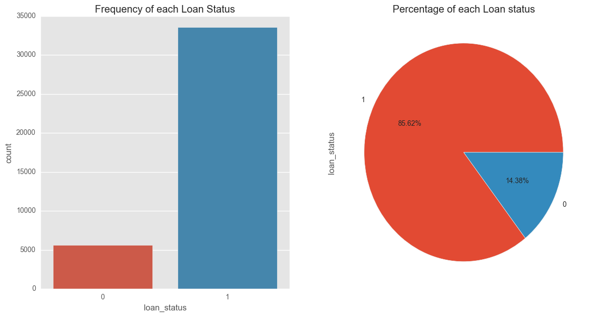
These plots indicate that a significant number of borrowers in our data set paid off their loan — 85.62% of loan borrowers paid off amount borrowed, while 14.38% unfortunately defaulted. It is these 'defaulters' that we're more interested identifying, since for the purposes of our model we're trying to find a way to maximize investment returns.
Not lending to these defaulters would help increase our returns, so we'll continue cleaning our data with an eye towards building a model that can identify likely defaulters at the point of application.
Remove Columns with only One Value
To wrap up this section, let's look for any columns that contain only one unique value and remove them. These columns won't be useful for the model since they don't add any information to each loan application. In addition, removing these columns will reduce the number of columns we'll need to explore further in the next stage.
The pandas Series method nunique() returns the number of unique values, excluding any null values. We can use apply this method across the data set to remove these columns in one easy step.
loans_2007 = loans_2007.loc[:,loans_2007.apply(pd.Series.nunique) != 1]Again, there may be some columns with more than one unique value, but one value that has insignificant frequency in the data set. Let's find and drop any columns with unique values that appear fewer than four times:
for col in loans_2007.columns:
    if (len(loans_2007[col].unique()) < 4):
    print(loans_2007[col].value_counts())
    print()
36 months 29096
60 months 10143
Name: term, dtype: int64
Not Verified 16845
Verified 12526
Source Verified 9868
Name: verification_status, dtype: int64
1 33586
0 5653
Name: loan_status, dtype: int64
n 39238
y 1
Name: pymnt_plan, dtype: int64
The payment plan column (pymnt_plan) has two unique values, 'y' and 'n', with 'y' occurring only once. Let's drop this column:
print(loans_2007.shape[1])
loans_2007 = loans_2007.drop('pymnt_plan', axis=1)
print("We've been able to reduce the features to => {}".format(loans_2007.shape[1]))
25
We've been able to reduce the features to => 24
Lastly, let's use pandas to save our freshly-cleaned DataFrame as a CSV file:
loans_2007.to_csv("processed_data/filtered_loans_2007.csv",index=False)Now we've got a much better data set to work with. But we're still not done with our data cleaning work, so let's keep at it!
Step 3: Preparing the Features for Machine Learning
In this section, we'll prepare the filtered_loans_2007.csv data for machine learning. We'll focus on handling missing values, converting categorical columns to numeric columns and removing any other extraneous columns.
We need to handle missing values and categorical features before feeding the data into a machine learning algorithm, because the mathematics underlying most machine learning models assumes that the data is numerical and contains no missing values. To reinforce this requirement, scikit-learn will return an error if you try to train a model using data that contain missing values or non-numeric values when working with models like linear regression and logistic regression.
Here's an outline of what we'll be doing in this stage:
- Handle Missing Values
- Investigate Categorical Columns
- Convert Categorical Columns To Numeric Features
- Map Ordinal Values To Integers
- Encode Nominal Values As Dummy Variables
- Convert Categorical Columns To Numeric Features
First though, let's load in the data from last section's final output:
filtered_loans = pd.read_csv('processed_data/filtered_loans_2007.csv')
print(filtered_loans.shape)
filtered_loans.head()
(39239, 24)Handle Missing Values
Let's compute the number of missing values and determine how to handle them. We can return the number of missing values across the DataFrame like this:
- First, use the Pandas DataFrame method
isnull()to return a DataFrame containing Boolean values:Trueif the original value is nullFalseif the original value isn't null
- Then, use the Pandas DataFrame method
sum()to calculate the number of null values in each column.
null_counts = filtered_loans.isnull().sum()
print("Number of null values in each column:\n{}".format(null_counts))
Number of null values in each column:
loan_amnt 0
term 0
installment 0
grade 0
emp_length  0
home_ownership 0
annual_inc 0
verification_status 0
loan_status 0
purpose 0
title 10
addr_state 0
dti 0
delinq_2yrs 0
earliest_cr_line 0
inq_last_6mths 0
open_acc 0
pub_rec 0
revol_bal 0
revol_util 50
total_acc 0
last_credit_pull_d 2
pub_rec_bankruptcies 697
fico_average 0
dtype: int64
Notice while most of the columns have 0 missing values, title has 9 missing values, revol_util has 48, and pub_rec_bankruptcies contains 675 rows with missing values.
Let's remove columns entirely where more than 1% (392) of the rows for that column contain a null value. In addition, we'll remove the remaining rows containing null values. This means we'll lose a bit of data, but in return keep some extra features to use for prediction (since we won't have to drop those columns).
We'll keep the title and revol_util columns, just removing rows containing missing values, but drop the pub_rec_bankruptcies column entirely since more than 1% of the rows have a missing value for this column.
Specifically, here's what we're going to do:
- Use the drop method to remove the pub_rec_bankruptcies column from filtered_loans.
- Use the dropna method to remove all rows from filtered_loans containing any missing values.
And here's how that looks in code.
filtered_loans = filtered_loans.drop("pub_rec_bankruptcies",axis=1)
filtered_loans = filtered_loans.dropna()
Note that there are a variety of ways to deal with missing values, and this is one of the most important steps in data cleaning for machine learning. Our Data Cleaning Advanced course for Python goes into a lot more depth on handling missing values when cleaning data and would be a great source for deeper learning on this topic.
For our purposes here, though, we're all set with this step, so let's move on to working with the categorical columns.
Investigate Categorical Columns
Our goal here is to end up with a data set that's ready for machine learning, meaning that it contains no missing values and that all values in columns are numeric (float or int data type).
We dealt with the missing values already, so let's now find out the number of columns that are of the object data type and figure out how we can make those values numeric.
print("Data types and their frequency\n{}".format(filtered_loans.dtypes.value_counts()))Data types and their frequency
float64 11
object 11
int64 1
dtype: int64We have 11 object columns that contain text which need to be converted into numeric features. Let's select just the object columns using the DataFrame method select_dtype, then display a sample row to get a better sense of how the values in each column are formatted.
object_columns_df = filtered_loans.select_dtypes(include=['object'])
print(object_columns_df.iloc[0])
term 36 months
grade B
emp_length 10+ years
home_ownership RENT
verification_status Verified
purpose credit_card
title Computer
addr_state AZ
earliest_cr_line Jan-1985
revol_util 83.7%
last_credit_pull_d Sep-2016
Name: 0, dtype: object
Notice that revol_util column contains numeric values, but is formatted as object. We learned from the description of columns in the preview DataFrame earlier that revol_util is a "revolving line utilization rate or the amount of credit the borrower is using relative to all available credit" (read more here). We need to format revol_util as a numeric value. Here's what we can do:
- Use the
str.rstrip()string method to strip the right trailing percent sign (On the resulting Series object, use theastype()method to convert to the typefloat. - Assign the new Series of float values back to the
revol_utilcolumn in thefiltered_loans.
filtered_loans['revol_util'] = filtered_loans['revol_util'].str.rstrip(
Moving on, these columns seem to represent categorical values:
home_ownership — home ownership status, can only be 1 of 4 categorical values according to the data dictionary.verification_status — indicates if income was verified by LendingClub.emp_length — number of years the borrower was employed upon time of application.term — number of payments on the loan, either 36 or 60.addr_state — borrower's state of residence.grade — LC assigned loan grade based on credit score.purpose — a category provided by the borrower for the loan request.title — loan title provided the borrower.
To be sure, lets confirm by checking the number of unique values in each of them.
Also, based on the first row's values for purpose and title, it appears these two columns reflect the same information. We'll explore their unique value counts separately to confirm if this is true.
Lastly, notice the first row's values for both earliest_cr_line and last_credit_pull_d columns contain date values that would require a good amount of feature engineering for them to be potentially useful:
earliest_cr_line — The month the borrower's earliest reported credit line was opened.last_credit_pull_d — The most recent month LendingClub pulled credit for this loan.
For some analyses, doing this feature engineering might well be worth it, but for the purposes of this tutorial we'll just remove these date columns from the DataFrame.
First, let's explore the unique value counts of the six columns that seem like they contain categorical values:
cols = ['home_ownership', 'grade','verification_status', 'emp_length', 'term', 'addr_state']
for name in cols:
print(name,':')
print(object_columns_df[name].value_counts(),'\n')
home_ownership :
RENT 18677
MORTGAGE 17381
OWN 3020
OTHER 96
NONE 3
Name: home_ownership, dtype: int64
grade :
B 11873
A 10062
C 7970
D 5194
E 2760
F 1009
G 309
Name: grade, dtype: int64
verification_status :
Not Verified 16809
Verified 12515
Source Verified 9853
Name: verification_status, dtype: int64
emp_length :
10+ years 8715
< 1 year 4542
2 years 4344
3 years 4050
4 years 3385
5 years 3243
1 year 3207
6 years 2198
7 years 1738
8 years 1457
9 years 1245
n/a 1053
Name: emp_length, dtype: int64
term :
36 months 29041
60 months 10136
Name: term, dtype: int64
addr_state :
CA 7019
NY 3757
FL 2831
TX 2693
NJ 1825
IL 1513
PA 1493
VA 1388
GA 1381
MA 1322
OH 1197
MD 1039
AZ 863
WA 830
CO 777
NC 772
CT 738
MI 718
MO 677
MN 608
NV 488
SC 469
WI 447
OR 441
AL 441
LA 432
KY 319
OK 294
KS 264
UT 255
AR 241
DC 211
RI 197
NM 187
WV 174
HI 170
NH 169
DE 113
MT 84
WY 83
AK 79
SD 61
VT 53
MS 19
TN 17
IN 9
ID 6
IA 5
NE 5
ME 3
Name: addr_state, dtype: int64
Most of these columns contain discrete categorical values which we can encode as dummy variables and keep. The addr_state column, however, contains too many unique values, so it's better to drop this.
Next, let's look at the unique value counts for the purpose and title columns to understand which columns we want to keep.
for name in ['purpose','title']:
print("Unique Values in column: {}\n".format(name))
print(filtered_loans[name].value_counts(),'\n')
Unique Values in column: purpose
debt_consolidation 18355
credit_card 5073
other 3921
home_improvement 2944
major_purchase 2178
small_business 1792
car 1534
wedding 940
medical 688
moving 580
vacation 377
house 372
educational 320
renewable_energy 103
Name: purpose, dtype: int64
Unique Values in column: title
Debt Consolidation 2142
Debt Consolidation Loan 1670
Personal Loan 650
Consolidation 501
debt consolidation 495
Credit Card Consolidation 354
Home Improvement 350
Debt consolidation 331
Small Business Loan 317
Credit Card Loan 310
Personal 306
Consolidation Loan 255
Home Improvement Loan 243
personal loan 231
personal 217
Loan 210
Wedding Loan 206
Car Loan 198
consolidation 197
Other Loan 187
Credit Card Payoff 153
Wedding 152
Major Purchase Loan 144
Credit Card Refinance 143
Consolidate 126
Medical 120
Credit Card 115
home improvement 109
My Loan 94
Credit Cards 92
...
toddandkim4ever 1
Remainder of down payment 1
Building a Financial Future 1
Higher interest payoff 1
Chase Home Improvement Loan 1
Sprinter Purchase 1
Refi credit card-great payment record 1
Karen's Freedom Loan 1
Business relocation and partner buyout 1
Update My New House 1
tito 1
florida vacation 1
Back to 0 1
Bye Bye credit card 1
britschool 1
Consolidation 16X60 1
Last Call 1
Want to be debt free in "3" 1
for excellent credit 1
loaney 1
jamal's loan 1
Refying Lending Club-I LOVE THIS PLACE! 1
Consoliation Loan 1
Personal/ Consolidation 1
Pauls Car 1
Road to freedom loan 1
Pay it off FINALLY! 1
MASH consolidation 1
Destination Wedding 1
Store Charge Card 1
Name: title, dtype: int64
It appears the purpose and title columns do contain overlapping information, but the purpose column contains fewer discrete values and is cleaner, so we'll keep it and drop title.
Lets drop the columns we've decided not to keep so far:
drop_cols = ['last_credit_pull_d','addr_state','title','earliest_cr_line']
filtered_loans = filtered_loans.drop(drop_cols,axis=1)
Convert Categorical Columns to Numeric Features
First, let's understand the two types of categorical features we have in our dataset and how we can convert each to numerical features:
- Ordinal values: these categorical values are in natural order. We can sort or order them either in increasing or decreasing order. For instance, we learned earlier that LendingClub grades loan applicants from A to G, and assigns each applicant a corresponding interest rate - grade A is least risky, grade B is riskier than A, and so on:
A < B < C < D < E < F < G ; where < means less risky than
- Nominal Values: these are regular categorical values. You can't order nominal values. For instance, while we can order loan applicants in the employment length column (
emp_length) based on years spent in the workforce:
year 1 < year 2 < year 3 ... < year N,
we can't do that with the column purpose. It wouldn't make sense to say:
car < wedding < education < moving < house
These are the columns we now have in our dataset:
- Ordinal Values
gradeemp_length
- Nominal Values _
home_ownership
verification_statuspurposeterm
There are different approaches to handle each of these two types. To map the ordinal values to integers, we can use the pandas DataFrame method replace() to map both grade and emp_length to appropriate numeric values:
mapping_dict = {
"emp_length": {
"10+ years": 10,
"9 years": 9,
"8 years": 8,
"7 years": 7,
"6 years": 6,
"5 years": 5,
"4 years": 4,
"3 years": 3,
"2 years": 2,
"1 year": 1,
"< 1 year": 0,
"n/a": 0
},
"grade":{
"A": 1,
"B": 2,
"C": 3,
"D": 4,
"E": 5,
"F": 6,
"G": 7
}
}
filtered_loans = filtered_loans.replace(mapping_dict)
filtered_loans[['emp_length','grade']].head()
Perfect! Let's move on to the Nominal Values. Converting nominal features into numerical features requires encoding them as dummy variables. The process will be:
- Use pandas'
get_dummies() method to return a new DataFrame containing a new column for each dummy variable.
- Use the
concat() method to add these dummy columns back to the original DataFrame.
- Drop the original columns entirely using the drop method.
Let's go ahead and encode the nominal columns that we have in our data set:
nominal_columns = ["home_ownership", "verification_status", "purpose", "term"]
dummy_df = pd.get_dummies(filtered_loans[nominal_columns])
filtered_loans = pd.concat([filtered_loans, dummy_df], axis=1)
filtered_loans = filtered_loans.drop(nominal_columns, axis=1)
filtered_loans.head()
To wrap things up, let's inspect our final output from this section to make sure all the features are of the same length, contain no null value, and are numerical. We'll use pandas's info method to inspect the filtered_loans DataFrame:
filtered_loans.info()
<class 'pandas.core.frame.dataframe'="">
Int64Index: 39177 entries, 0 to 39238
Data columns (total 39 columns):
loan_amnt 39177 non-null float64
installment 39177 non-null float64
grade 39177 non-null int64
emp_length 39177 non-null int64
annual_inc 39177 non-null float64
loan_status 39177 non-null int64
dti 39177 non-null float64
delinq_2yrs 39177 non-null float64
inq_last_6mths 39177 non-null float64
open_acc 39177 non-null float64
pub_rec 39177 non-null float64
revol_bal 39177 non-null float64
revol_util 39177 non-null float64
total_acc 39177 non-null float64
fico_average 39177 non-null float64
home_ownership_MORTGAGE 39177 non-null uint8
home_ownership_NONE 39177 non-null uint8
home_ownership_OTHER 39177 non-null uint8
home_ownership_OWN 39177 non-null uint8
home_ownership_RENT 39177 non-null uint8
verification_status_Not Verified 39177 non-null uint8
verification_status_Source Verified 39177 non-null uint8
verification_status_Verified 39177 non-null uint8
purpose_car 39177 non-null uint8
purpose_credit_card 39177 non-null uint8
purpose_debt_consolidation 39177 non-null uint8
purpose_educational 39177 non-null uint8
purpose_home_improvement 39177 non-null uint8
purpose_house 39177 non-null uint8
purpose_major_purchase 39177 non-null uint8
purpose_medical 39177 non-null uint8
purpose_moving 39177 non-null uint8
purpose_other 39177 non-null uint8
purpose_renewable_energy 39177 non-null uint8
purpose_small_business 39177 non-null uint8
purpose_vacation 39177 non-null uint8
purpose_wedding 39177 non-null uint8
term_ 36 months 39177 non-null uint8
term_ 60 months 39177 non-null uint8
dtypes: float64(12), int64(3), uint8(24)
memory usage: 5.7 MB
</class>
That all looks good! Congratulations, we've just cleaned a large data set for machine learning, and added some valuable data cleaning skills to our repertoire in the process.
There's still an important final task we need to complete, though!
Save to CSV
It is a good practice to store the final output of each section or stage of your workflow in a separate csv file. One of the benefits of this practice is that it helps us to make changes in our data processing flow without having to recalculate everything.
As we did previously, we can store our DataFrame as a CSV using the handy pandas to_csv() function.
filtered_loans.to_csv("processed_data/cleaned_loans_2007.csv",index=False)
Next Steps
In this post, we've covered the basic steps required to work through a large data set, cleaning and preparing the data for a machine learning project. But there's lots more to learn, and there are plenty of different directions you might choose to go from here.
If you're feeling comfortable with your data cleaning skills and you'd like to work more with this data set, check out our interactive machine learning walkthrough course which covers the next steps in working with this Lending Club data.
If you'd like to keep working on your data cleaning skills, check out one (or more) of our interactive data cleaning courses to dive deeper into this crucial data science skill:
- Data Cleaning and Analysis course (Python)
- Advanced Data Cleaning course (Python)
- Data Cleaning (R)
About the original author, Daniel Osei: After first reading about Machine Learning on Quora in 2015, Daniel became excited at the prospect of an area that could combine his love of Mathematics and Programming. After reading this article on how to learn data science, Daniel started following the steps, eventually joining Dataquest to learn Data Science with us in in April 2016. We'd like to thank Daniel for his hard work, and generously letting us publish this post. This post was updated by a Dataquest editor in June, 2019.