Continuous integration of machine learning models with ease.ml/ci: towards a rigorous yet practical treatment Renggli et al., SysML’19
Developing machine learning models is no different from developing traditional software, in the sense that it is also a full life cycle involving design, implementation, tuning, testing, and deployment. As machine learning models are used in more task-critical applications and are more tightly integrated with traditional software stacks, it becomes increasingly important for the ML development life cycle also to be managed following systematic, rigit engineering discipline.
I didn’t find this an easy paper to follow at all points, but the question it addresses is certainly interesting: what does a continuous integration testing environment look like for a machine learning model? ease.ml/ci is a CI system for machine learning, and it has to take into account two main differences from a regular CI test suite:
- Machine learning is inherently probabilistic , so test conditions are evaluated with respect to an
-reliability requirement, where
is the probability of a valid test, and
is the error tolerance.
- By getting pass/fail feedback from the CI server, the model can adapt to the test set used in the CI environment, leading to it overfitting over time. So test sets used for CI have a ‘shelf-life’, after which they need to be refreshed.
The tricky parts then, are (a) figuring out how many samples you need to achieve a given level of
Use cases
Examples of use cases collected across both academia and industry include:
- F1: The model must meet at least a given quality threshold (lower bound worst case quality).
- F2: Each new model should be better than the previous one (incremental quality improvement)
- F3: Models released to production must show significant quality improvements, i.e., better than the previous model by some given threshold (significant quality milestones)
- F4: Stability of predictions across models: the predictions made by the new model should not change significantly from those made by the previous model (no significant changes)
- Hybrids of the above, especially incremental quality improvement combined with no significant changes.
Overview
ease.ml/ci can integrate with an existing CI server (Travis in the implementation), and provides a DSL for specifying model tests. The user must also provide the N test examples to be used in the CI environment. Given a test script which includes conditions for 
ease.ml/ci will calculate how large N needs to be on behalf of the user.
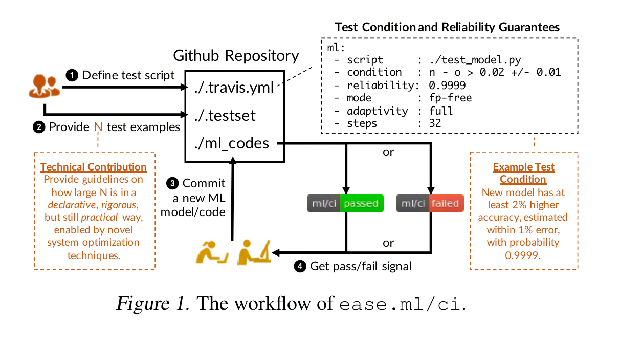
When the current test set loses its statistical power due to repeated evaluation, ease.ml/ci will raise an alarm (e.g. send an email to a provided email address) to indicate that a new test set is now required.
At the first glance of the problem, there seems to exist a trivial implementation: for each committed model, draw N labeled data points from the testset, get an
-estimate of the accuracy of the new model, and test whether it satisfies the test conditions or not. The challenge of this strategy is the practicality associated with the label complexity (i.e., how large N is)…
If you’re not careful, N can be sufficiently large so as to make the scheme impractical. The techniques used by ease.ml/ci are designed to keep the number of samples required to achieve the desired level of reliability down to a minimum. Even so, we could be talking about a lot of labels: “from our experience working with different users, we observe that providing 30,000 to 60,000 labels for every 32 model evaluations seems reasonable for many users…”. That’s around 1,000 to 2,000 labeled test examples per test suite run! A test set of 30-60K labelled data items typically takes those users around a day to collect, and with one commit/day will last about a month. Anything above this level is considered ‘impractical.’
Controlling adaptation
A prominent difference between
ease.ml/ciand traditional continuous integration systems is that the statistical power of a test dataset will decrease when the result of whether a new model passes the continuous integration test is released to the developer.
Here comes the part I’m still struggling to get my head around. A test script includes an adaptivity specification which can take on values full, none, and firstChange. With full adaptivity things work as you would expect, with the developer learning whether or not the build passed on the CI server. If you specify none here though, the result of the CI test is hidden from the developer (but can be made visible to some other group). But how then does the developer know that the model needs further improvement??? Yes we can keep using the same testset for longer this way, but other than as a guard on production release it seems to me we get much diminished utility from it. With the firstChange strategy the developer gets immediate pass/fail feedback, but as soon as the result changes from the previous run (e.g. a failing build is now passing) the system requires a new testset.
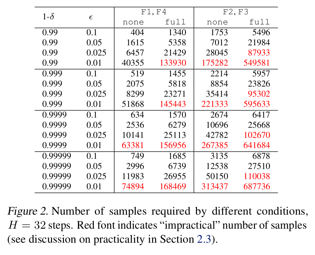
The table below shows estimations of the number of samples required by ease.ml under the none and full adaptivity strategies for various test criteria (F1-F4), test validity probabilities 

The test script language
ease.ml/ci adds an ml section to a Travis CI configuration file that looks like this:
ml:
  - script      : ./test_model.py
  - condition   : n - o < 0.02 +/- 0.01
  - reliability : 0.9999
  - mode        : fp-free
  - adaptivity  : full
  - steps       : 32
The condition clause can range over three variables, n, o, and d, where n is the accuracy of the new model, o is the accuracy of the old model, and d is the percentage of predictions that are different under the new model as compared to the old model.
The steps parameter controls how many times the user wishes to be able to reuse a test set. ease.ml/ci will take this into account when calculating how large (N) the testset needs to be.
The mode parameter controls whether it is more important to be false-positive free (fp-free) or false-negative free (fn-free).
Give a script, ease.ml/ci will calculate the number of testset examples the user needs to provide. Given a script and a CI test execution history, ease.ml/ci will also generate alarms when the testset needs to be refreshed.
Here’s how the common use cases described earlier are typically mapped into the DSL:
Lower bound worst case quality (F1)
...
- condition  : n > [c] +/- [epsilon]
- adaptivity : none
- mode       : fn-free
Incremental quality improvement (F2)
...
- condition  : n - o > [c] +/- [epsilon]
- adaptivity : full
- mode       : fp-free
Significant quality milestones (F3)
...
- condition  : n -o > [c] +/- [epsilon]
- adaptivity : firstChange
- mode       : fp-free
No significant changes (F4)
...
- condition  : d < [c] +/- [epsilon]
- adaptivity : full | none
- mode       : fn-free
(where c is large).
Hybrid
For hybrid scenarios the condition clause can be expressed as condition_one /\ condition_two. (Because && and and were taken??).
Minimising the number of required samples
Estimates for the number of required samples are derived using the standard Hoeffding inequality in the non-adaptive case, and a technique similar to Ladder (Blum & Hardt, 2015) in the adaptive case. As we saw earlier in figure 2, this can support a number of common conditions within the bounds of practicality. As we get stricter on accuracy (ε) though, things get especially tough when using the fully adaptive strategy:
…none of the adaptive strategy [cases from figure 2] are practical up to 1 accuracy point, a level of tolerance that is important for many task-critical applications of machine learning.
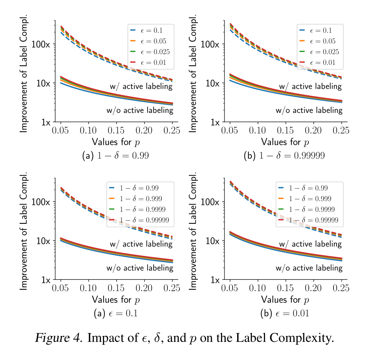
ease.ml/ci contains a number of optimisations for common test conditions though which can improve the sample size required considerably – by up to two orders of magnitude in some cases. Details of these optimisations can be found in section 4 of the paper, and rely on two technical observations:
- When the new model and the old model are close in their predictions, Bennett’s inequality can be used.
- To estimate the difference in predictions between the old model and the new model you don’t need labels – a sample from an unlabelled dataset can be used instead. Then to estimate e.g.
n - owhen 10% of data points have different predictions requires only 10% of the whole dataset to be labelled. This strategy is called active labelling.
Evaluation
The sample size optimisations can reduce the number of labels required by 10x without active labelling, and by an additional further 10x when active labelling is used.
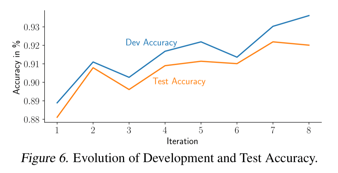
The following evaluation shows CI build status evolution for models from the SemEval-2019 Task 3 competition (classify emotions of a user utterance as Happy, Sad, Angry, or Other), under three different test scenarios.
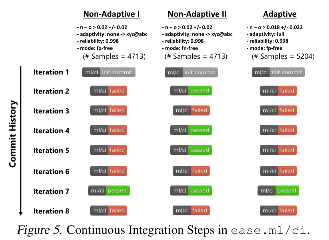
In all cases the model from iteration 7 will be chosen for deployment, even though the developer believed iteration 8 to be an improvement. This iteration gives better accuracy on the development test set, but not on the CI test set.