The convolutional layer in convolutional neural networks systematically applies filters to an input and creates output feature maps.
Although the convolutional layer is very simple, it is capable of achieving sophisticated and impressive results. Nevertheless, it can be challenging to develop an intuition for how the shape of the filters impacts the shape of the output feature map and how related configuration hyperparameters such as padding and stride should be configured.
In this tutorial, you will discover an intuition for filter size, the need for padding, and stride in convolutional neural networks.
After completing this tutorial, you will know:
- How filter size or kernel size impacts the shape of the output feature map.
- How the filter size creates a border effect in the feature map and how it can be overcome with padding.
- How the stride of the filter on the input image can be used to downsample the size of the output feature map.
Kick-start your project with my new book Deep Learning for Computer Vision, including step-by-step tutorials and the Python source code files for all examples.
Let’s get started.

A Gentle Introduction to Padding and Stride for Convolutional Neural Networks
Photo by Red~Star, some rights reserved.
Tutorial Overview
This tutorial is divided into five parts; they are:
- Convolutional Layer
- Problem of Border Effects
- Effect of Filter Size (Kernel Size)
- Fix the Border Effect Problem With Padding
- Downsample Input With Stride
Want Results with Deep Learning for Computer Vision?
Take my free 7-day email crash course now (with sample code).
Click to sign-up and also get a free PDF Ebook version of the course.
Convolutional Layer
In a convolutional neural network, a convolutional layer is responsible for the systematic application of one or more filters to an input.
The multiplication of the filter to the input image results in a single output. The input is typically three-dimensional images (e.g. rows, columns and channels), and in turn, the filters are also three-dimensional with the same number of channels and fewer rows and columns than the input image. As such, the filter is repeatedly applied to each part of the input image, resulting in a two-dimensional output map of activations, called a feature map.
Keras provides an implementation of the convolutional layer called a Conv2D.
It requires that you specify the expected shape of the input images in terms of rows (height), columns (width), and channels (depth) or [rows, columns, channels].
The filter contains the weights that must be learned during the training of the layer. The filter weights represent the structure or feature that the filter will detect and the strength of the activation indicates the degree to which the feature was detected.
The layer requires that both the number of filters be specified and that the shape of the filters be specified.
We can demonstrate this with a small example. In this example, we define a single input image or sample that has one channel and is an eight pixel by eight pixel square with all 0 values and a two-pixel wide vertical line in the center.
|
1 2 3 4 5 6 7 8 9 10 11 |
# define input data data = [[0, 0, 0, 1, 1, 0, 0, 0], [0, 0, 0, 1, 1, 0, 0, 0], [0, 0, 0, 1, 1, 0, 0, 0], [0, 0, 0, 1, 1, 0, 0, 0], [0, 0, 0, 1, 1, 0, 0, 0], [0, 0, 0, 1, 1, 0, 0, 0], [0, 0, 0, 1, 1, 0, 0, 0], [0, 0, 0, 1, 1, 0, 0, 0]] data = asarray(data) data = data.reshape(1, 8, 8, 1) |
Next, we can define a model that expects input samples to have the shape (8, 8, 1) and has a single hidden convolutional layer with a single filter with the shape of three pixels by three pixels.
|
1 2 3 4 5 |
# create model model = Sequential() model.add(Conv2D(1, (3,3), input_shape=(8, 8, 1))) # summarize model model.summary() |
The filter is initialized with random weights as part of the initialization of the model. We will overwrite the random weights and hard code our own 3×3 filter that will detect vertical lines.
That is the filter will strongly activate when it detects a vertical line and weakly activate when it does not. We expect that by applying this filter across the input image, the output feature map will show that the vertical line was detected.
|
1 2 3 4 5 6 7 |
# define a vertical line detector detector = [[[[0]],[[1]],[[0]]], [[[0]],[[1]],[[0]]], [[[0]],[[1]],[[0]]]] weights = [asarray(detector), asarray([0.0])] # store the weights in the model model.set_weights(weights) |
Next, we can apply the filter to our input image by calling the predict() function on the model.
|
1 2 |
# apply filter to input data yhat = model.predict(data) |
The result is a four-dimensional output with one batch, a given number of rows and columns, and one filter, or [batch, rows, columns, filters].
We can print the activations in the single feature map to confirm that the line was detected.
|
1 2 3 4 |
# enumerate rows for r in range(yhat.shape[1]): # print each column in the row print([yhat[0,r,c,0] for c in range(yhat.shape[2])]) |
Tying all of this together, the complete example is listed below.
|
1 2 3 4 5 6 7 8 9 10 11 12 13 14 15 16 17 18 19 20 21 22 23 24 25 26 27 28 29 30 31 32 33 |
# example of using a single convolutional layer from numpy import asarray from keras.models import Sequential from keras.layers import Conv2D # define input data data = [[0, 0, 0, 1, 1, 0, 0, 0], [0, 0, 0, 1, 1, 0, 0, 0], [0, 0, 0, 1, 1, 0, 0, 0], [0, 0, 0, 1, 1, 0, 0, 0], [0, 0, 0, 1, 1, 0, 0, 0], [0, 0, 0, 1, 1, 0, 0, 0], [0, 0, 0, 1, 1, 0, 0, 0], [0, 0, 0, 1, 1, 0, 0, 0]] data = asarray(data) data = data.reshape(1, 8, 8, 1) # create model model = Sequential() model.add(Conv2D(1, (3,3), input_shape=(8, 8, 1))) # summarize model model.summary() # define a vertical line detector detector = [[[[0]],[[1]],[[0]]], [[[0]],[[1]],[[0]]], [[[0]],[[1]],[[0]]]] weights = [asarray(detector), asarray([0.0])] # store the weights in the model model.set_weights(weights) # apply filter to input data yhat = model.predict(data) # enumerate rows for r in range(yhat.shape[1]): # print each column in the row print([yhat[0,r,c,0] for c in range(yhat.shape[2])]) |
Running the example first summarizes the structure of the model.
Of note is that the single hidden convolutional layer will take the 8×8 pixel input image and will produce a feature map with the dimensions of 6×6. We will go into why this is the case in the next section.
We can also see that the layer has 10 parameters, that is nine weights for the filter (3×3) and one weight for the bias.
Finally, the feature map is printed. We can see from reviewing the numbers in the 6×6 matrix that indeed the manually specified filter detected the vertical line in the middle of our input image.
|
1 2 3 4 5 6 7 8 9 10 11 12 13 14 15 16 17 |
_________________________________________________________________ Layer (type) Output Shape Param # ================================================================= conv2d_1 (Conv2D) (None, 6, 6, 1) 10 ================================================================= Total params: 10 Trainable params: 10 Non-trainable params: 0 _________________________________________________________________ [0.0, 0.0, 3.0, 3.0, 0.0, 0.0] [0.0, 0.0, 3.0, 3.0, 0.0, 0.0] [0.0, 0.0, 3.0, 3.0, 0.0, 0.0] [0.0, 0.0, 3.0, 3.0, 0.0, 0.0] [0.0, 0.0, 3.0, 3.0, 0.0, 0.0] [0.0, 0.0, 3.0, 3.0, 0.0, 0.0] |
Problem of Border Effects
In the previous section, we defined a single filter with the size of three pixels high and three pixels wide (rows, columns).
We saw that the application of the 3×3 filter, referred to as the kernel size in Keras, to the 8×8 input image resulted in a feature map with the size of 6×6.
That is, the input image with 64 pixels was reduced to a feature map with 36 pixels. Where did the other 28 pixels go?
The filter is applied systematically to the input image. It starts at the top left corner of the image and is moved from left to right one pixel column at a time until the edge of the filter reaches the edge of the image.
For a 3×3 pixel filter applied to a 8×8 input image, we can see that it can only be applied six times, resulting in the width of six in the output feature map.
For example, let’s work through each of the six patches of the input image (left) dot product (“.” operator) the filter (right):
|
1 2 3 |
0, 0, 0 0, 1, 0 0, 0, 0 . 0, 1, 0 = 0 0, 0, 0 0, 1, 0 |
Moved right one pixel:
|
1 2 3 |
0, 0, 1 0, 1, 0 0, 0, 1 . 0, 1, 0 = 0 0, 0, 1 0, 1, 0 |
Moved right one pixel:
|
1 2 3 |
0, 1, 1 0, 1, 0 0, 1, 1 . 0, 1, 0 = 3 0, 1, 1 0, 1, 0 |
Moved right one pixel:
|
1 2 3 |
1, 1, 0 0, 1, 0 1, 1, 0 . 0, 1, 0 = 3 1, 1, 0 0, 1, 0 |
Moved right one pixel:
|
1 2 3 |
1, 0, 0 0, 1, 0 1, 0, 0 . 0, 1, 0 = 0 1, 0, 0 0, 1, 0 |
Moved right one pixel:
|
1 2 3 |
0, 0, 0 0, 1, 0 0, 0, 0 . 0, 1, 0 = 0 0, 0, 0 0, 1, 0 |
That gives us the first row and each column of the output feature map:
|
1 |
0.0, 0.0, 3.0, 3.0, 0.0, 0.0 |
The reduction in the size of the input to the feature map is referred to as border effects. It is caused by the interaction of the filter with the border of the image.
This is often not a problem for large images and small filters but can be a problem with small images. It can also become a problem once a number of convolutional layers are stacked.
For example, below is the same model updated to have two stacked convolutional layers.
This means that a 3×3 filter is applied to the 8×8 input image to result in a 6×6 feature map as in the previous section. A 3×3 filter is then applied to the 6×6 feature map.
|
1 2 3 4 5 6 7 8 9 |
# example of stacked convolutional layers from keras.models import Sequential from keras.layers import Conv2D # create model model = Sequential() model.add(Conv2D(1, (3,3), input_shape=(8, 8, 1))) model.add(Conv2D(1, (3,3))) # summarize model model.summary() |
Running the example summarizes the shape of the output from each layer.
We can see that the application of filters to the feature map output of the first layer, in turn, results in a smaller 4×4 feature map.
This can become a problem as we develop very deep convolutional neural network models with tens or hundreds of layers. We will simply run out of data in our feature maps upon which to operate.
|
1 2 3 4 5 6 7 8 9 10 11 |
_________________________________________________________________ Layer (type) Output Shape Param # ================================================================= conv2d_1 (Conv2D) (None, 6, 6, 1) 10 _________________________________________________________________ conv2d_2 (Conv2D) (None, 4, 4, 1) 10 ================================================================= Total params: 20 Trainable params: 20 Non-trainable params: 0 _________________________________________________________________ |
Effect of Filter Size (Kernel Size)
Different sized filters will detect different sized features in the input image and, in turn, will result in differently sized feature maps.
It is common to use 3×3 sized filters, and perhaps 5×5 or even 7×7 sized filters, for larger input images.
For example, below is an example of the model with a single filter updated to use a filter size of 5×5 pixels.
|
1 2 3 4 5 6 7 8 |
# example of a convolutional layer from keras.models import Sequential from keras.layers import Conv2D # create model model = Sequential() model.add(Conv2D(1, (5,5), input_shape=(8, 8, 1))) # summarize model model.summary() |
Running the example demonstrates that the 5×5 filter can only be applied to the 8×8 input image 4 times, resulting in a 4×4 feature map output.
|
1 2 3 4 5 6 7 8 9 |
_________________________________________________________________ Layer (type) Output Shape Param # ================================================================= conv2d_1 (Conv2D) (None, 4, 4, 1) 26 ================================================================= Total params: 26 Trainable params: 26 Non-trainable params: 0 _________________________________________________________________ |
It may help to further develop the intuition of the relationship between filter size and the output feature map to look at two extreme cases.
The first is a filter with the size of 1×1 pixels.
|
1 2 3 4 5 6 7 8 |
# example of a convolutional layer from keras.models import Sequential from keras.layers import Conv2D # create model model = Sequential() model.add(Conv2D(1, (1,1), input_shape=(8, 8, 1))) # summarize model model.summary() |
Running the example demonstrates that the output feature map has the same size as the input, specifically 8×8. This is because the filter only has a single weight (and a bias).
|
1 2 3 4 5 6 7 8 9 |
_________________________________________________________________ Layer (type) Output Shape Param # ================================================================= conv2d_1 (Conv2D) (None, 8, 8, 1) 2 ================================================================= Total params: 2 Trainable params: 2 Non-trainable params: 0 _________________________________________________________________ |
The other extreme is a filter with the same size as the input, in this case, 8×8 pixels.
|
1 2 3 4 5 6 7 8 |
# example of a convolutional layer from keras.models import Sequential from keras.layers import Conv2D # create model model = Sequential() model.add(Conv2D(1, (8,8), input_shape=(8, 8, 1))) # summarize model model.summary() |
Running the example, we can see that, as you might expect, there is one weight for each pixel in the input image (64 + 1 for the bias) and that the output is a feature map with a single pixel.
|
1 2 3 4 5 6 7 8 9 |
_________________________________________________________________ Layer (type) Output Shape Param # ================================================================= conv2d_1 (Conv2D) (None, 1, 1, 1) 65 ================================================================= Total params: 65 Trainable params: 65 Non-trainable params: 0 _________________________________________________________________ |
Now that we are familiar with the effect of filter sizes on the size of the resulting feature map, let’s look at how we can stop losing pixels.
Fix the Border Effect Problem With Padding
By default, a filter starts at the left of the image with the left-hand side of the filter sitting on the far left pixels of the image. The filter is then stepped across the image one column at a time until the right-hand side of the filter is sitting on the far right pixels of the image.
An alternative approach to applying a filter to an image is to ensure that each pixel in the image is given an opportunity to be at the center of the filter.
By default, this is not the case, as the pixels on the edge of the input are only ever exposed to the edge of the filter. By starting the filter outside the frame of the image, it gives the pixels on the border of the image more of an opportunity for interacting with the filter, more of an opportunity for features to be detected by the filter, and in turn, an output feature map that has the same shape as the input image.
For example, in the case of applying a 3×3 filter to the 8×8 input image, we can add a border of one pixel around the outside of the image. This has the effect of artificially creating a 10×10 input image. When the 3×3 filter is applied, it results in an 8×8 feature map. The added pixel values could have the value zero value that has no effect with the dot product operation when the filter is applied.
|
1 2 3 |
x, x, x 0, 1, 0 x, 0, 0 . 0, 1, 0 = 0 x, 0, 0 0, 1, 0 |
The addition of pixels to the edge of the image is called padding.
In Keras, this is specified via the “padding” argument on the Conv2D layer, which has the default value of ‘valid‘ (no padding). This means that the filter is applied only to valid ways to the input.
The ‘padding‘ value of ‘same‘ calculates and adds the padding required to the input image (or feature map) to ensure that the output has the same shape as the input.
The example below adds padding to the convolutional layer in our worked example.
|
1 2 3 4 5 6 7 8 |
# example a convolutional layer with padding from keras.models import Sequential from keras.layers import Conv2D # create model model = Sequential() model.add(Conv2D(1, (3,3), padding='same', input_shape=(8, 8, 1))) # summarize model model.summary() |
Running the example demonstrates that the shape of the output feature map is the same as the input image: that the padding had the desired effect.
|
1 2 3 4 5 6 7 8 9 |
_________________________________________________________________ Layer (type) Output Shape Param # ================================================================= conv2d_1 (Conv2D) (None, 8, 8, 1) 10 ================================================================= Total params: 10 Trainable params: 10 Non-trainable params: 0 _________________________________________________________________ |
The addition of padding allows the development of very deep models in such a way that the feature maps do not dwindle away to nothing.
The example below demonstrates this with three stacked convolutional layers.
|
1 2 3 4 5 6 7 8 9 10 |
# example a deep cnn with padding from keras.models import Sequential from keras.layers import Conv2D # create model model = Sequential() model.add(Conv2D(1, (3,3), padding='same', input_shape=(8, 8, 1))) model.add(Conv2D(1, (3,3), padding='same')) model.add(Conv2D(1, (3,3), padding='same')) # summarize model model.summary() |
Running the example, we can see that with the addition of padding, the shape of the output feature maps remains fixed at 8×8 even three layers deep.
|
1 2 3 4 5 6 7 8 9 10 11 12 13 |
_________________________________________________________________ Layer (type) Output Shape Param # ================================================================= conv2d_1 (Conv2D) (None, 8, 8, 1) 10 _________________________________________________________________ conv2d_2 (Conv2D) (None, 8, 8, 1) 10 _________________________________________________________________ conv2d_3 (Conv2D) (None, 8, 8, 1) 10 ================================================================= Total params: 30 Trainable params: 30 Non-trainable params: 0 _________________________________________________________________ |
Downsample Input With Stride
The filter is moved across the image left to right, top to bottom, with a one-pixel column change on the horizontal movements, then a one-pixel row change on the vertical movements.
The amount of movement between applications of the filter to the input image is referred to as the stride, and it is almost always symmetrical in height and width dimensions.
The default stride or strides in two dimensions is (1,1) for the height and the width movement, performed when needed. And this default works well in most cases.
The stride can be changed, which has an effect both on how the filter is applied to the image and, in turn, the size of the resulting feature map.
For example, the stride can be changed to (2,2). This has the effect of moving the filter two pixels right for each horizontal movement of the filter and two pixels down for each vertical movement of the filter when creating the feature map.
We can demonstrate this with an example using the 8×8 image with a vertical line (left) dot product (“.” operator) with the vertical line filter (right) with a stride of two pixels:
|
1 2 3 |
0, 0, 0 0, 1, 0 0, 0, 0 . 0, 1, 0 = 0 0, 0, 0 0, 1, 0 |
Moved right two pixels:
|
1 2 3 |
0, 1, 1 0, 1, 0 0, 1, 1 . 0, 1, 0 = 3 0, 1, 1 0, 1, 0 |
Moved right two pixels:
|
1 2 3 |
1, 0, 0 0, 1, 0 1, 0, 0 . 0, 1, 0 = 0 1, 0, 0 0, 1, 0 |
We can see that there are only three valid applications of the 3×3 filters to the 8×8 input image with a stride of two. This will be the same in the vertical dimension.
This has the effect of applying the filter in such a way that the normal feature map output (6×6) is down-sampled so that the size of each dimension is reduced by half (3×3), resulting in 1/4 the number of pixels (36 pixels down to 9).
The stride can be specified in Keras on the Conv2D layer via the ‘stride‘ argument and specified as a tuple with height and width.
The example demonstrates the application of our manual vertical line filter on the 8×8 input image with a convolutional layer that has a stride of two.
|
1 2 3 4 5 6 7 8 9 10 11 12 13 14 15 16 17 18 19 20 21 22 23 24 25 26 27 28 29 30 31 32 33 |
# example of vertical line filter with a stride of 2 from numpy import asarray from keras.models import Sequential from keras.layers import Conv2D # define input data data = [[0, 0, 0, 1, 1, 0, 0, 0], [0, 0, 0, 1, 1, 0, 0, 0], [0, 0, 0, 1, 1, 0, 0, 0], [0, 0, 0, 1, 1, 0, 0, 0], [0, 0, 0, 1, 1, 0, 0, 0], [0, 0, 0, 1, 1, 0, 0, 0], [0, 0, 0, 1, 1, 0, 0, 0], [0, 0, 0, 1, 1, 0, 0, 0]] data = asarray(data) data = data.reshape(1, 8, 8, 1) # create model model = Sequential() model.add(Conv2D(1, (3,3), strides=(2, 2), input_shape=(8, 8, 1))) # summarize model model.summary() # define a vertical line detector detector = [[[[0]],[[1]],[[0]]], [[[0]],[[1]],[[0]]], [[[0]],[[1]],[[0]]]] weights = [asarray(detector), asarray([0.0])] # store the weights in the model model.set_weights(weights) # apply filter to input data yhat = model.predict(data) # enumerate rows for r in range(yhat.shape[1]): # print each column in the row print([yhat[0,r,c,0] for c in range(yhat.shape[2])]) |
Running the example, we can see from the summary of the model that the shape of the output feature map will be 3×3.
Applying the handcrafted filter to the input image and printing the resulting activation feature map, we can see that, indeed, the filter still detected the vertical line, and can represent this finding with less information.
Downsampling may be desirable in some cases where deeper knowledge of the filters used in the model or of the model architecture allows for some compression in the resulting feature maps.
|
1 2 3 4 5 6 7 8 9 10 11 12 13 14 |
_________________________________________________________________ Layer (type) Output Shape Param # ================================================================= conv2d_1 (Conv2D) (None, 3, 3, 1) 10 ================================================================= Total params: 10 Trainable params: 10 Non-trainable params: 0 _________________________________________________________________ [0.0, 3.0, 0.0] [0.0, 3.0, 0.0] [0.0, 3.0, 0.0] |
Further Reading
This section provides more resources on the topic if you are looking to go deeper.
Posts
Books
- Chapter 9: Convolutional Networks, Deep Learning, 2016.
- Chapter 5: Deep Learning for Computer Vision, Deep Learning with Python, 2017.
API
Summary
In this tutorial, you discovered an intuition for filter size, the need for padding, and stride in convolutional neural networks.
Specifically, you learned:
- How filter size or kernel size impacts the shape of the output feature map.
- How the filter size creates a border effect in the feature map and how it can be overcome with padding.
- How the stride of the filter on the input image can be used to downsample the size of the output feature map.
Do you have any questions?
Ask your questions in the comments below and I will do my best to answer.




Hi, suppose I use stacked filters. Will the numbers within the filters same? For example:
model.add(Conv2D(1, (3,3), padding=’same’, input_shape=(8, 8, 1)))
model.add(Conv2D(1, (3,3), padding=’same’))
model.add(Conv2D(1, (3,3), padding=’same’))
How does the filter look in line 2 and line 3. Does the filter have the same values as in line 1? In general it will be good to know how to construct the filters?
Each filter will have different random numbers when initialized, and after training will have a different representation – will detect different features.
“For example, the stride can be changed to (2,2). This has the effect of moving the filter two pixels left for each horizontal movement of the filter and two pixels down for each vertical movement of the filter when creating the feature map.”
Correction: “For example, the stride can be changed to (2,2). This has the effect of moving the filter two pixels right for each horizontal movement of the filter and two pixels down for each vertical movement of the filter when creating the feature map.”
Thanks, fixed.
Is there any specific equation to compute size of feature map given the input size (n*n), padding size (p) and stride (s)?
Yes, perhaps check this document:
https://arxiv.org/abs/1603.07285
Nice, detailed tutorial. Thanks.
It just sounded odd to me the terminology of “dot product”, which is not appropriate and misleading.
Thanks.
More on matrix math here:
https://machinelearningmastery.com/introduction-matrices-machine-learning/
Thanks a lot, Jason. Stumbled on to your post as part of my extra reading for a TF course. Really helped me understand the intuition and math behind conv filters.
Thanks.
Thanks, I’m happy to hear that.
Note that in the stride example, you run the risk of completely missing the vertical line, if it is too thin. For example, if a single input row can be represented as:
[0,0,0,0,1,0,0,0]
then the strident Convolutional filter will dance right over it, because it is going to stop at column 1, 3, and 5. Note that column 4 possesses the vertical line segment.
Yes, it is possible. It’s just a contrived example.
Thanks Jason,
this blog was really helpful in giving a detailed explanation of zero padding and stride .and how all these works….All of your articles are always very helpful in undersatding the things in deeper…..it will be better if also add the formula of calculating the size of feature map in this post…
Thanks!
Great suggestion.
Great explanation
Thanks Jason!
Thanks. Hope you enjoyed it.
thanks for such Wonderful information, hope you will help us to get out of the problem by shareing concepts like this.
Thanks for the great article.
I am working on a deep learning assignment that uses images as input.
I’ve already done tutorials on mnist and ImageNet, but their input images are very small.
Since practical input images are large, we need to scale or convolution them.
I would like to choose convolution, but I don’t know how to determine the size of the filter.
Is there any discussion on what percentage of the original image the filter should be within, or should it be 3×3 and have more layers?
Increasing the size of the filter seems to speed up the dimension reduction, but it also seems to lose some information.
If we reduce the size of the filter, we may be able to keep the amount of information, but the speed of dimension reduction will be slower and processing will take longer.
I think these are trade-offs, but is there an appropriate way to approach this?
Hi Ogawa! You may find the following interesting:
https://machinelearningmastery.com/how-to-visualize-filters-and-feature-maps-in-convolutional-neural-networks/
Thanks for your comment.
I read your article about CNN visualization.
I have done this before on mnist numbers.
It was just like doing a mosaic on the numbers.
You can really feel the effect of CNNs when you can recognize them as numbers, even though the mosaic process reduces the amount of information in the image.
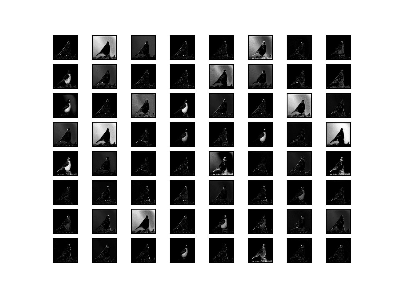
The image discussed in the article is a bird, so you can barely recognize it as a bird until block 3, but it gives you a good idea of what part of the image CNN is observing and at what granularity.
Now, James.
I am trying to figure out what should be done about the size of the input image.
The article you referred to seems to be scaling the image to 224×224 to fit the input layer of VGG16.
As a starting point, I have actually tried a similar method.
Here, I think it would be better to try convolution rather than scaling to improve the accuracy with the same data.
Is there any indication as to what filter size (and layer) expansion I should try then?
What do you think? Is there much discussion about these?
Or am I not explaining myself well enough?
I hope to get some comments.
for this piece of codes
inp = tf.zeros([64, 64, 3])
inp = tf.expand_dims(inp, axis=0)
inp = tf.keras.layers.Conv2D(16, (2, 2), (2, 2), padding=’same’)(inp)
print(inp.shape)
(1, 32, 32, 16)
the inp shape does not change when I change the kernel size to (3, 3) or (5, 5). Could you please explain this?
Because you’re using “same” padding. Each “pixel” in your output just computed differently (with a larger kernel) but still the same stride, etc.